Research note: hyperparameter uncertainty and identifiability

optimize_gp() returns point estimates of the hyperparameters. gp_hyperparameter_uncertainty() adds a Laplace approximation: the inverse of the observed information I = -\nabla^2 \ell(\hat\eta) on the optimizer’s coordinate scale \eta (logarithms of positive parameters), computed by central differences of the analytical gradient. This note checks whether those standard errors describe the variability of the estimates, and shows how the same curvature reveals hyperparameters that the data cannot identify.

Do the standard errors match the spread of the estimates?

The script below, inst/examples/hyperparameter-uncertainty.R, simulates 200 data sets of 60 noisy observations of a known RBF process, estimates the variance, length scale, and noise variance on each, and compares the standard deviation of the estimates across data sets with the reported standard errors. It is run as-is to produce this page.

# Do reported standard errors match the spread of the estimates?
#
# Simulate 200 data sets from a known Gaussian process, estimate its
# hyperparameters on each with optimize_gp(), and compare the standard errors
# that gp_hyperparameter_uncertainty() reports with the standard deviation of
# the estimates across data sets. Everything is on the optimizer's log scale.

library(gaussianprocesses)

truth <- rbf_kernel(variance = 1, length_scale = 0.8)
true_noise <- 0.04
x <- seq(0, 10, length.out = 60)
true_values <- log(c(variance = 1, length_scale = 0.8, noise_variance = 0.04))

replicates <- lapply(
  seq_len(200),
  function(seed) {
    simulated <- simulate_gp_data(
      x,
      truth,
      noise_variance = true_noise,
      seed = seed
    )
    model <- optimize_gp(
      x,
      simulated$observed,
      kernel = truth,
      noise_variance = true_noise,
      n_starts = 1
    )
    uncertainty <- gp_hyperparameter_uncertainty(model)

    list(
      estimate = uncertainty$parameters$coordinate_estimate,
      standard_error = uncertainty$parameters$standard_error,
      poorly_identified = uncertainty$poorly_identified
    )
  }
)

estimates <- do.call(rbind, lapply(replicates, `[[`, "estimate"))
standard_errors <- do.call(rbind, lapply(replicates, `[[`, "standard_error"))
colnames(estimates) <- colnames(standard_errors) <- names(true_values)

z <- stats::qnorm(0.975)
covered <- abs(sweep(estimates, 2, true_values)) <= z * standard_errors

study <- data.frame(
  parameter = names(true_values),
  spread_of_estimates = apply(estimates, 2, stats::sd),
  # The scaled median absolute deviation equals the standard deviation for
  # normal estimates but ignores their tails.
  robust_spread = apply(estimates, 2, stats::mad),
  median_standard_error = apply(standard_errors, 2, stats::median),
  coverage_95 = colMeans(covered),
  row.names = NULL
)
study
#>        parameter spread_of_estimates robust_spread median_standard_error
#> 1       variance           0.5484313     0.5235059             0.4790420
#> 2   length_scale           0.1666347     0.1489557             0.1326517
#> 3 noise_variance           0.2121662     0.2263299             0.2141936
#>   coverage_95
#> 1       0.900
#> 2       0.905
#> 3       0.950

# Monte Carlo standard error of the coverage of 200 intervals.
sqrt(0.95 * 0.05 / 200)
#> [1] 0.01541104
sum(vapply(replicates, `[[`, logical(1), "poorly_identified"))
#> [1] 2

The reported standard errors are of the right size but somewhat too small for the kernel parameters at this sample size: the median standard error is 13% below the spread of the variance estimates and 20% below that of the length scale, while for the noise variance they agree. Correspondingly, nominal 95% intervals cover the true values in 90%, 90%, and 95% of data sets; the Monte Carlo standard error of each coverage is 1.5 percentage points.

The Laplace approximation assumes that the log likelihood is quadratic in \eta, so that the estimates are normal. With 60 observations the length-scale estimates are heavy-tailed and the variance estimates skewed; the robust spread, which ignores the tails, is closer to the standard errors but still larger. The approximation is a useful summary of how precisely the data determine each parameter, but when intervals matter the profile likelihood (gp_profile_likelihood()) makes no quadratic assumption.

Poorly identified hyperparameters

Some hyperparameters cannot be determined by the data however the estimate is computed. For a Matérn kernel with smoothness \nu observed densely on a bounded domain (infill asymptotics), only the combination \sigma^2 / \ell^{2\nu} is consistently estimable (Zhang, 2004): data cannot tell a larger variance with a longer length scale from a smaller variance with a shorter one. The log likelihood then has a ridge, and the observed information is nearly singular along it.

Compare 100 observations of a Matérn 3/2 process with length scale 3 on [0, 1], within one length scale, with 100 observations of one with length scale 5 on [0, 100], twenty length scales:

fit_matern <- function(range, length_scale) {
  x <- seq(0, range, length.out = 100)
  truth <- matern32_kernel(variance = 1, length_scale = length_scale)
  simulated <- simulate_gp_data(x, truth, noise_variance = 1e-4, seed = 1)
  optimize_gp(
    x,
    simulated$observed,
    kernel = truth,
    noise_variance = 1e-4,
    optimize_noise = FALSE,
    n_starts = 1
  )
}

infill <- fit_matern(1, 3)
wide <- fit_matern(100, 5)

gp_hyperparameter_uncertainty(infill)
#> Hyperparameter uncertainty (Laplace approximation on the optimizer scale)
#>     parameter estimate coordinate standard_error lower 95% upper 95%
#>      variance  0.42269        log          1.470   0.02351     7.600
#>  length_scale  2.76200        log          0.585   0.87820     8.687
#>   condition number of the information: 65.9
#>   weakest log-scale combination: standard deviation 1.57
#>   poorly identified along: 0.94 variance + 0.35 length_scale (coordinate scale)
gp_hyperparameter_uncertainty(wide)
#> Hyperparameter uncertainty (Laplace approximation on the optimizer scale)
#>     parameter estimate coordinate standard_error lower 95% upper 95%
#>      variance  0.61816        log          0.346    0.3135     1.219
#>  length_scale  4.43980        log          0.141    3.3680     5.853
#>   condition number of the information: 46.3
#>   weakest log-scale combination: standard deviation 0.37

The infill fit is flagged as poorly identified. The direction along which the likelihood is flattest, 0.94, 0.35 in (log variance, log length scale), is the ridge \sigma^2 / \ell^3 = constant, whose direction is (3, 1) / \sqrt{10} \approx (0.95, 0.32). The flag fires because the standard deviation along the least determined combination of log-scale parameters exceeds \log 2: that combination is known only to within a factor of two. The condition number alone would not show it, because the curvature across the ridge is small too.

The profile likelihood shows the same thing without the quadratic approximation. For each fixed variance it maximizes the likelihood over the length scale:

profile <- function(model) {
  estimate <- model$kernel$parameters$variance
  gp_profile_likelihood(
    model,
    "variance",
    values = estimate * exp(seq(-2.5, 2.5, length.out = 21))
  )
}
infill_profile <- profile(infill)
wide_profile <- profile(wide)

plot(
  infill_profile$value / infill$kernel$parameters$variance,
  infill_profile$deviance,
  type = "l",
  log = "x",
  ylim = c(0, 8),
  xlab = "variance relative to its estimate",
  ylab = "deviance"
)
lines(
  wide_profile$value / wide$kernel$parameters$variance,
  wide_profile$deviance,
  lty = 2
)
abline(h = stats::qchisq(0.95, 1), col = "grey60", lty = 3)
legend(
  "top",
  legend = c("infill", "twenty length scales"),
  lty = c(1, 2),
  bty = "n"
)

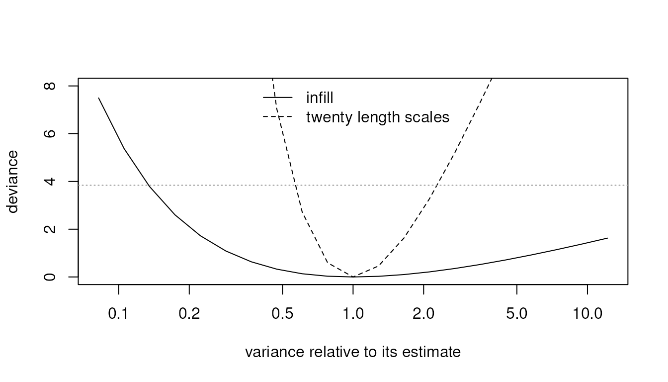
Values whose deviance lies below the dotted line, \chi^2_{1, 0.95}, form an approximate 95% interval. For the wide design it runs from about half to about twice the estimate. For the infill design it runs from about a seventh of the estimate to beyond the right edge of the plot, more than ten times it: the data say little about the variance on its own.

Several optima

The likelihood can also have several separate maxima, for example for changepoint locations or spectral-mixture frequencies. optimize_gp() groups its starts by the optimum they reach, and summary() reports how many distinct optima the starts found and how far below the best they are. One optimum reached from every start is reassuring; distinct optima with large gaps mean that the result depends on the starts, and distinct optima with nearly equal likelihoods but different parameters suggest a ridge.

Reference

Zhang, H. (2004). Inconsistent estimation and asymptotically equal interpolations in model-based geostatistics. Journal of the American Statistical Association, 99(465), 250–261.