Research note: binary classification with latent Gaussian processes

A Gaussian-process classifier places a Gaussian process prior on a latent function f and observes binary responses through a link, \Pr(y_i = 1 \mid f) = \pi(f(x_i)), \qquad \pi(f) = \frac{1}{1 + e^{-f}} \ \text{(logit)} \quad \text{or} \quad \pi(f) = \Phi(f) \ \text{(probit)}. fit_latent_gp() and optimize_latent_gp() fit it with bernoulli_likelihood() and the Laplace approximation to the posterior of f. This note shows the workflow, explains what the predicted probabilities mean, and checks their calibration in a simulation from a known Gaussian-process classifier.

Labels and fitting

Responses may be 0/1 numbers, logical values, or a two-level factor. As in glm(), the second level of a factor is the event coded 1, and every predicted probability refers to it.

set.seed(4)
x <- sort(runif(120, 0, 10))
latent <- 2.5 * sin(x) + 0.5 * cos(3 * x)
labels <- factor(
  ifelse(runif(120) < plogis(latent), "positive", "negative"),
  levels = c("negative", "positive")
)

model <- optimize_latent_gp(x, labels, rbf_kernel(), bernoulli_likelihood(),
                            n_starts = 2)
model
#> Latent Gaussian-process model (Laplace approximation)
#>   observations: 120
#>   input dimensions: 1
#>   likelihood: BernoulliLikelihood(link=logit)
#>   mean: ZeroMean()
#>   Newton iterations: 5 (converged)
#>   approximate log marginal likelihood: -62.88884
#>   numerical jitter: 0
#>   optimization: converged (L-BFGS-B, analytical gradient)
#>   kernel:
#>     RBF(variance=3.96531, length_scale=1.22556)
model$response_levels
#> [1] "negative" "positive"

predict_latent_gp() returns the latent posterior and, for Bernoulli likelihoods, the predictive probability of the event with an interval for the class probability \pi(f(x_*)) itself.

grid <- seq(0, 10, length.out = 300)
prediction <- predict_latent_gp(model, grid)

plot(grid, prediction$probability, type = "n", ylim = c(0, 1.35),
     xlab = "x", ylab = "Pr(positive)", yaxt = "n")
axis(2, at = seq(0, 1, by = 0.2))
polygon(c(grid, rev(grid)),
        c(prediction$probability_interval[, 1],
          rev(prediction$probability_interval[, 2])),
        col = "grey85", border = NA)
lines(grid, prediction$probability, lwd = 2)
lines(grid, plogis(2.5 * sin(grid) + 0.5 * cos(3 * grid)), lty = 2)
points(x, as.numeric(labels == "positive"), pch = "|", cex = 0.7)
legend("topleft", c("predictive probability", "true probability",
                    "95% interval of the class probability"),
       lty = c(1, 2, NA), lwd = c(2, 1, NA), pch = c(NA, NA, 15),
       col = c("black", "black", "grey85"), bty = "n", cex = 0.8,
       ncol = 2)

What the predicted probability is

Under the Laplace approximation the latent value at a new input is Gaussian, f_* \mid y \approx N(\mu_*, \sigma_*^2), and the predictive probability averages the link over it: \Pr(y_* = 1 \mid y) = \int \pi(f_*)\, N(f_* \mid \mu_*, \sigma_*^2)\, df_*. For the probit link this is \Phi(\mu_* / \sqrt{1 + \sigma_*^2}) exactly; for the logit link it is computed by Gauss–Hermite quadrature, accurate to 10^{-10} with the default 40 nodes for \sigma_*^2 \le 3. The averaging pulls the probability towards 1/2 where the latent function is uncertain. Two common shortcuts ignore part of it:

mean_grid <- seq(-10, 10, by = 0.05)
shortcut_errors <- t(sapply(c(0.25, 1, 4), function(variance) {
  exact <- likelihood_predictive(
    bernoulli_likelihood(), mean_grid, rep(variance, length(mean_grid)),
    quadrature_order = 80
  )$probability
  c(
    variance = variance,
    plug_in = max(abs(plogis(mean_grid) - exact)),
    mackay = max(abs(plogis(mean_grid / sqrt(1 + pi * variance / 8)) - exact))
  )
}))
round(shortcut_errors, 4)
#>      variance plug_in mackay
#> [1,]     0.25  0.0113 0.0014
#> [2,]     1.00  0.0391 0.0046
#> [3,]     4.00  0.1062 0.0101

The plug-in probability \pi(\mu_*) ignores the latent variance, and MacKay’s approximation \sigma(\kappa \mu_*) with \kappa = (1 + \pi \sigma_*^2 / 8)^{-1/2} replaces the logistic function by a scaled probit. The package computes the integral instead.

probability_interval is a different quantity: the interval for the class probability \pi(f_*), whose uncertainty comes from f_*. Because the link is increasing it is the link applied to the latent interval, and the probability draws of sample_gp_posterior() describe its joint uncertainty at several inputs.

Scoring probability forecasts

gp_holdout_scores() scores a classifier on held-out data with the log loss and Brier score (proper scoring rules), the ROC AUC (discrimination only), and reliability data with the expected calibration error.

training <- seq(1, 120, by = 2)
held_out <- setdiff(seq_len(120), training)
fit <- fit_latent_gp(x[training], labels[training], model$kernel,
                     bernoulli_likelihood())
scores <- gp_holdout_scores(fit, x[held_out], labels[held_out], n_bins = 5)
scores
#> Classification scores for 60 responses (base rate 0.6167)
#>   log loss: 0.4677
#>   Brier score: 0.1472
#>   ROC AUC: 0.8684
#>   expected calibration error: 0.08691 (5 occupied bins)
scores$reliability
#>   bin lower upper  n mean_probability observed_frequency standard_error
#> 1   1   0.0   0.2  7        0.1791588          0.1428571      0.1449438
#> 2   2   0.2   0.4 14        0.2670429          0.2857143      0.1182404
#> 3   3   0.4   0.6 11        0.5084852          0.5454545      0.1507340
#> 4   4   0.6   0.8 15        0.7226298          0.8666667      0.1155958
#> 5   5   0.8   1.0 13        0.8359984          1.0000000      0.1026964

Simulation study

The script below, inst/examples/gp-classification-study.R, draws 300 data sets from a known Gaussian-process classifier, fits each on 80 training inputs, and scores the forecasts of 200 test responses. It compares the true probabilities (the oracle), the predictive probabilities with the true and with estimated hyperparameters, and the plug-in probability. It is run as-is to produce this page.

# Calibration of Gaussian-process classification on data from a known GP
# classifier.
#
# Each replicate draws a latent function f from a Gaussian process with an
# RBF kernel (variance 4, length scale 1) at 280 uniform inputs on [0, 10],
# and binary responses y ~ Bernoulli(plogis(f)). The first 80 are for
# training, the other 200 for testing. Four forecasts of the test responses
# are scored:
#   oracle     plogis(f), the true probabilities;
#   known      the predictive probability with the true hyperparameters;
#   plug-in    plogis() of the latent mean with the true hyperparameters,
#              which ignores the latent uncertainty;
#   estimated  the predictive probability with hyperparameters estimated
#              by optimize_latent_gp().
# Scores are averaged over replicates, with Monte Carlo standard errors, and
# the test forecasts of all replicates are pooled for reliability curves.

library(gaussianprocesses)

n_replicates <- 300
n_training <- 80
n_test <- 200
kernel <- rbf_kernel(variance = 4, length_scale = 1)
methods <- c("oracle", "known", "plug-in", "estimated")

set.seed(20261007)
scores <- list()
forecasts <- list()
estimates <- matrix(NA_real_, n_replicates, 2,
                    dimnames = list(NULL, c("variance", "length_scale")))
bound_warnings <- 0L

for (replicate in seq_len(n_replicates)) {
  x <- stats::runif(n_training + n_test, 0, 10)
  f <- drop(sample_gp_prior(x, kernel)$latent)
  y <- stats::rbinom(length(x), 1, stats::plogis(f))
  training <- seq_len(n_training)
  test <- n_training + seq_len(n_test)

  known <- fit_latent_gp(x[training], y[training], kernel,
                         bernoulli_likelihood())
  known_prediction <- predict_latent_gp(known, x[test])

  estimated <- withCallingHandlers(
    optimize_latent_gp(x[training], y[training], rbf_kernel(),
                       bernoulli_likelihood(), n_starts = 1),
    gaussianprocesses_bound_warning = function(condition) {
      bound_warnings <<- bound_warnings + 1L
      invokeRestart("muffleWarning")
    }
  )
  estimates[replicate, ] <- kernel_parameters(estimated$kernel,
                                              flatten = TRUE)

  probability <- list(
    oracle = stats::plogis(f[test]),
    known = known_prediction$probability,
    `plug-in` = stats::plogis(known_prediction$mean),
    estimated = predict_latent_gp(estimated, x[test])$probability
  )

  for (method in methods) {
    result <- gp_classification_scores(y[test], probability[[method]])
    scores[[length(scores) + 1L]] <- data.frame(
      replicate = replicate,
      method = method,
      brier_score = result$summary[["brier_score"]],
      log_loss = result$summary[["log_loss"]],
      ece = result$summary[["ece"]]
    )
    forecasts[[length(forecasts) + 1L]] <- data.frame(
      method = method,
      probability = probability[[method]],
      observed = y[test]
    )
  }
}

scores <- do.call(rbind, scores)
forecasts <- do.call(rbind, forecasts)

# Means over replicates with Monte Carlo standard errors.
summarize <- function(values) {
  c(mean = mean(values), se = stats::sd(values) / sqrt(length(values)))
}
study <- do.call(rbind, lapply(methods, function(method) {
  rows <- scores[scores$method == method, ]
  brier <- summarize(rows$brier_score)
  log_loss <- summarize(rows$log_loss)
  ece <- summarize(rows$ece)
  data.frame(
    method = method,
    brier_score = brier[["mean"]],
    brier_se = brier[["se"]],
    log_loss = log_loss[["mean"]],
    log_loss_se = log_loss[["se"]],
    ece = ece[["mean"]],
    ece_se = ece[["se"]]
  )
}))

# Paired differences within replicates, whose standard errors are much
# smaller than those of the scores themselves.
paired <- function(method, baseline) {
  difference <- function(score) {
    values <- scores[[score]][scores$method == method] -
      scores[[score]][scores$method == baseline]
    c(mean(values), stats::sd(values) / sqrt(n_replicates))
  }
  brier <- difference("brier_score")
  log_loss <- difference("log_loss")

  data.frame(
    comparison = paste(method, "-", baseline),
    brier_score = brier[[1L]],
    brier_se = brier[[2L]],
    log_loss = log_loss[[1L]],
    log_loss_se = log_loss[[2L]]
  )
}
differences <- rbind(
  paired("known", "oracle"),
  paired("plug-in", "known"),
  paired("estimated", "known")
)

# Pooled reliability curves: test forecasts of every replicate in ten
# equal-width bins.
reliability <- do.call(rbind, lapply(methods, function(method) {
  rows <- forecasts[forecasts$method == method, ]
  bins <- gp_classification_scores(rows$observed, rows$probability)$reliability
  cbind(method = method, bins)
}))
reliability$z <- (reliability$observed_frequency -
                    reliability$mean_probability) / reliability$standard_error

# Calibration of the pooled forecasts: the ECE of all test forecasts
# together, and the largest bin deviation in standard errors.
pooled <- do.call(rbind, lapply(methods, function(method) {
  rows <- forecasts[forecasts$method == method, ]
  bins <- reliability[reliability$method == method, ]
  data.frame(
    method = method,
    ece = gp_classification_scores(rows$observed, rows$probability)$
      summary[["ece"]],
    largest_deviation = max(abs(bins$z))
  )
}))

print(study, digits = 3)
#>      method brier_score brier_se log_loss log_loss_se    ece  ece_se
#> 1    oracle       0.151  0.00191    0.461     0.00496 0.0618 0.00107
#> 2     known       0.166  0.00202    0.502     0.00493 0.0869 0.00156
#> 3   plug-in       0.165  0.00209    0.501     0.00521 0.0852 0.00155
#> 4 estimated       0.169  0.00211    0.511     0.00514 0.0910 0.00169
print(differences, digits = 3)
#>          comparison brier_score brier_se log_loss log_loss_se
#> 1    known - oracle    0.014682 0.000578  0.04136    0.001483
#> 2   plug-in - known   -0.000293 0.000111 -0.00127    0.000456
#> 3 estimated - known    0.003707 0.000387  0.00960    0.001009
print(pooled, digits = 3)
#>      method     ece largest_deviation
#> 1    oracle 0.00370              2.15
#> 2     known 0.01748              7.27
#> 3   plug-in 0.00474              3.30
#> 4 estimated 0.01265              4.55
cat("median estimates:", round(apply(estimates, 2, stats::median), 2),
    "\nbound warnings:", bound_warnings, "\n")
#> median estimates: 3.71 1.13 
#> bound warnings: 0

Scores

Even the oracle has a Brier score of 0.151: the responses are random given the true probabilities. With the true hyperparameters the predictive probabilities add 0.015 (Monte Carlo standard error 0.0006) to the Brier score and 0.041 to the log loss, the price of learning f from 80 noisy labels. Estimating the hyperparameters costs a further 0.0037 (0.0004) in Brier score; their median estimates, 3.71 for the variance and 1.13 for the length scale, are close to the true 4 and 1.

The differences are paired within data sets, so their standard errors are much smaller than those of the scores.

Calibration

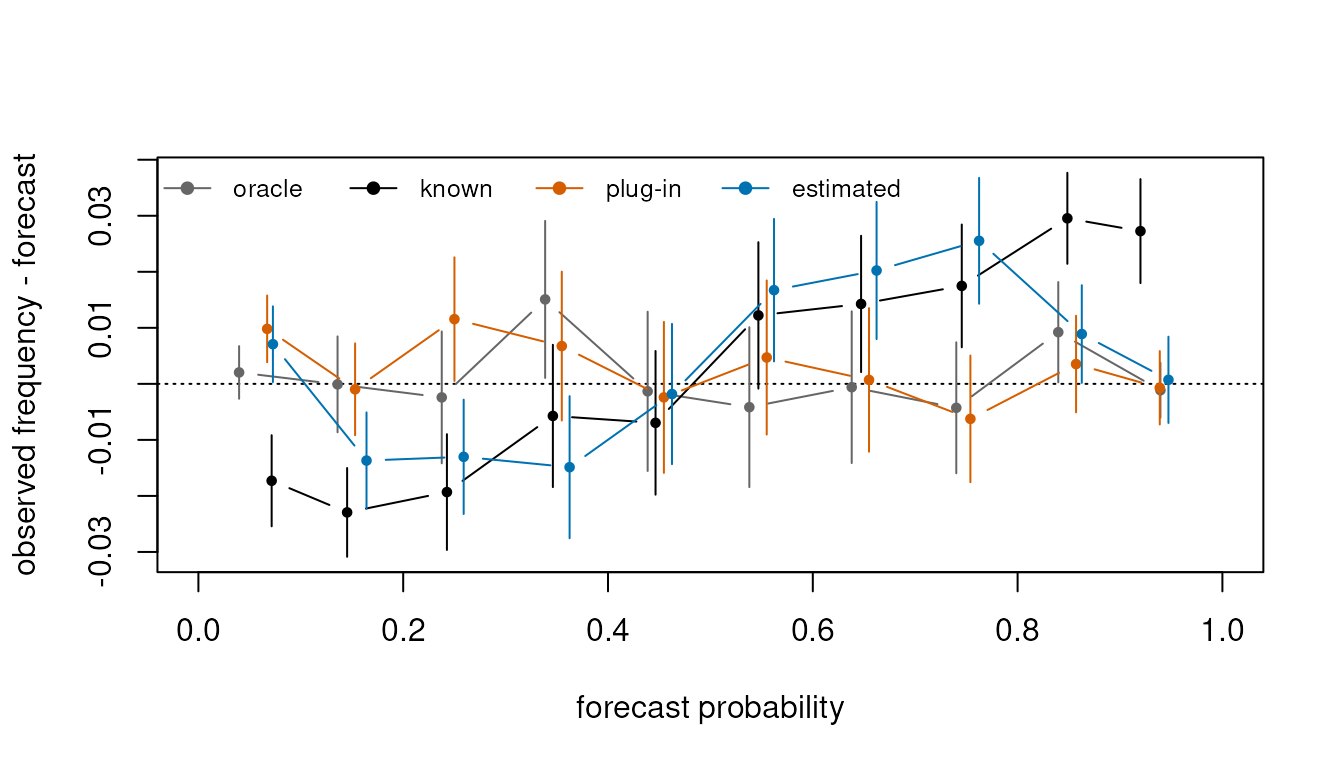
Pooling the test forecasts of all data sets gives reliability curves with small binomial standard errors. The figure shows each bin’s observed frequency minus its mean forecast, which is zero for calibrated forecasts. The oracle stays within 2.2 standard errors of zero in every bin, as a calibrated forecast should. The Laplace predictive probabilities with the true hyperparameters do not: they are too close to 1/2, by up to 7.3 standard errors, with observed frequencies below the forecast for small probabilities and above it for large ones. The plug-in probability, which does not average over the latent uncertainty, is better calibrated (largest deviation 3.3 standard errors) and even slightly better in Brier score, by 0.00029 (0.0001), and in log loss, by 0.0013 (0.0005).

This is a property of the Laplace approximation, not of the averaging. The exact posterior predictive probability is calibrated when the model is right, as it is here. But the posterior of f given binary data is skewed, and its mode, around which the Laplace approximation is centred, lies closer to zero than its mean (Kuss and Rasmussen, 2005). Averaging the link over the approximation then shrinks the probabilities further towards 1/2, while the plug-in happens to offset the shrinkage of the mode. The effect is small in the proper scores and visible only in large pooled reliability curves; approximations that match the posterior mean, such as expectation propagation, would reduce it. The package reports the predictive probability because it is the quantity the model defines, and the plug-in has no such interpretation.

The expected calibration error of a single data set of 200 forecasts is dominated by sampling noise: even the oracle averages 0.062. Pooled over all data sets the noise is far smaller, and the ECE separates the forecasts: 0.0037 for the oracle against 0.017 with the true hyperparameters.

Separable classes

When the classes are separable, larger signal variances let the latent function separate them ever more sharply, and the approximate marginal likelihood keeps increasing up to very large variances.

separable_x <- 1:20
separable_y <- as.numeric(separable_x > 10)

unbounded <- optimize_latent_gp(separable_x, separable_y, rbf_kernel(),
                                bernoulli_likelihood(), n_starts = 1)
kernel_parameters(unbounded$kernel, flatten = TRUE)
#>     variance length_scale 
#>  1810.494750     5.542229

The estimate is far larger than any variance that overlapping classes would support. With an upper bound the search stops there, and a warning of class gaussianprocesses_bound_warning says that the bound determined the estimate:

bounded <- withCallingHandlers(
  optimize_latent_gp(separable_x, separable_y, rbf_kernel(),
                     bernoulli_likelihood(), n_starts = 1, upper = 100),
  gaussianprocesses_bound_warning = function(condition) {
    message("Warning: ", conditionMessage(condition))
    invokeRestart("muffleWarning")
  }
)
#> Warning: Optimized parameter(s) at a bound of the search: variance (upper). The approximate marginal likelihood may increase beyond it. For binary responses a signal variance at its upper bound usually means that the classes are separable, so that larger variances keep fitting them better; the bound then determines the fit.
bounded$optimization$at_bound
#> [1] "variance (upper)"

Validation and scope

The test suite checks the Laplace fits against an independent implementation, the gplite package, when it is installed: with the same kernel and jitter, the latent modes agree within 10^{-6}, as do the approximate log marginal likelihoods and the latent predictions. ?fit_latent_gp reports the error of the Laplace approximation to the marginal likelihood against tensor-product quadrature.

Multi-class (softmax) classification is not supported; it needs a vector of latent functions per input and is left for a later version.

References

Kuss, M. and Rasmussen, C. E. (2005). Assessing approximate inference for binary Gaussian process classification. Journal of Machine Learning Research, 6, 1679–1704.

MacKay, D. J. C. (1992). The evidence framework applied to classification networks. Neural Computation, 4(5), 720–736.

Rasmussen, C. E. and Williams, C. K. I. (2006). Gaussian Processes for Machine Learning. MIT Press. Chapter 3.