Derivatives of Covariance Kernels

Why derivatives

Hyperparameters are estimated by maximizing the log marginal likelihood. With C = K(\theta) + \Sigma_\varepsilon and \alpha = C^{-1}\tilde y, its derivative with respect to a kernel parameter is

\frac{\partial}{\partial \theta_j} \log p(y \mid X, \theta) = \frac{1}{2} \operatorname{tr}\!\left( \left(\alpha\alpha^\top - C^{-1}\right) \frac{\partial K}{\partial \theta_j} \right).

Everything specific to the kernel is in \partial K / \partial \theta_j. This vignette derives these matrices for every kernel in the package; kernel_gradient() computes them, and optimize_gp() uses them through log_marginal_likelihood_gradient().

Kernels can also be differentiated with respect to their inputs. Those derivatives are the covariances of the derivative of the process, and give the posterior gradient of the latent function; they also let a model condition on observed derivatives. They are derived in the last parts, Derivatives with respect to the inputs and Derivative observations.

Log parameters

Every kernel parameter is strictly positive, and the optimizer already works with \eta_j = \log \theta_j. Derivatives are therefore taken with respect to log parameters:

\frac{\partial K}{\partial \eta_j} = \theta_j \frac{\partial K}{\partial \theta_j}.

This is also convenient algebraically. If K is proportional to \theta_j, then \partial K / \partial \eta_j = K, and powers of \theta_j differentiate to integer multiples.

Scaled distances

For inputs x, x' \in \mathbb{R}^D and length scales \ell_1, \ldots, \ell_D, define the per-dimension terms and the scaled squared distance

s_d = \frac{(x_d - x'_d)^2}{\ell_d^2}, \qquad r^2 = \sum_{d=1}^D s_d.

Because s_d is proportional to \ell_d^{-2},

\frac{\partial s_d}{\partial \log \ell_d} = -2 s_d, \qquad \frac{\partial r^2}{\partial \log \ell_d} = -2 s_d.

With a single length scale \ell shared by all dimensions, \partial r^2 / \partial \log \ell = -2 r^2: the shared derivative is the sum of the ARD derivatives.

The variance parameter

Every kernel has the form k = \sigma^2 h, where h does not depend on \sigma^2. Hence

\frac{\partial k}{\partial \log \sigma^2} = k.

This holds for all eight kernels, including the linear and white-noise kernels, whose only parameter is the variance.

Stationary kernels

The RBF, Matérn, and rational-quadratic kernels have the form k = \sigma^2 f(r^2). By the chain rule,

\frac{\partial k}{\partial \log \ell_d} = \sigma^2 f'(r^2)\, \frac{\partial r^2}{\partial \log \ell_d} = g \, s_d, \qquad g = -2 \sigma^2 f'(r^2).

Only the radial factor g depends on the kernel. Each g can be written through k itself, so the implementation reuses the covariance values and never restates a kernel formula.

RBF

With f = \exp(-r^2/2), f' = -f/2, so

g = \sigma^2 f = k, \qquad \frac{\partial k}{\partial \log \ell_d} = k \, s_d.

Matérn 1/2

With f = e^{-r} and r = \sqrt{r^2}, f'(r^2) = -e^{-r} / (2r), so

g = \frac{\sigma^2 e^{-r}}{r} = \frac{k}{r}.

The factor is singular at r = 0, but the product is not: s_d \le r^2 gives g\, s_d \le k\, r \to 0. Coincident inputs therefore have zero length-scale derivative.

Matérn 3/2

With f = (1 + \sqrt{3} r) e^{-\sqrt{3} r}, \mathrm{d}f/\mathrm{d}r = -3 r e^{-\sqrt{3} r}, so f'(r^2) = -\tfrac{3}{2} e^{-\sqrt{3} r} and

g = 3 \sigma^2 e^{-\sqrt{3} r} = \frac{3k}{1 + \sqrt{3} r}.

Matérn 5/2

With f = (1 + \sqrt{5} r + \tfrac{5}{3} r^2) e^{-\sqrt{5} r}, \mathrm{d}f/\mathrm{d}r = -\tfrac{5}{3} r (1 + \sqrt{5} r) e^{-\sqrt{5} r}, so

g = \frac{5}{3} \sigma^2 (1 + \sqrt{5} r) e^{-\sqrt{5} r} = \frac{5}{3}\, k\, \frac{1 + \sqrt{5} r}{1 + \sqrt{5} r + \tfrac{5}{3} r^2}.

Rational quadratic

Write u = 1 + r^2 / (2\alpha), so f = u^{-\alpha}. Then f'(r^2) = -\tfrac{1}{2} u^{-\alpha - 1} and

g = \sigma^2 u^{-\alpha - 1} = \frac{k}{u}.

For the shape parameter, \log k = \log \sigma^2 - \alpha \log u and \partial u / \partial \alpha = -r^2 / (2\alpha^2), which give

\frac{\partial k}{\partial \log \alpha} = \alpha\, k\, \frac{\partial \log k}{\partial \alpha} = k \left( \frac{r^2}{2u} - \alpha \log u \right).

The implementation evaluates \log u as log1p(r^2 / (2 * alpha)), which stays accurate when r^2 / (2\alpha) is small.

Periodic kernel

With \delta_d = x_d - x'_d, a_d = \pi \delta_d / p, and

q_d = \frac{\sin^2 a_d}{\ell_d^2}, \qquad k = \sigma^2 \exp\!\left(-2 \sum_d q_d\right),

the length scales again enter through \ell_d^{-2}, so \partial q_d / \partial \log \ell_d = -2 q_d and

\frac{\partial k}{\partial \log \ell_d} = 4 k\, q_d.

For the period, \partial a_d / \partial \log p = -a_d and \partial \sin^2 a_d / \partial a_d = \sin 2 a_d, so

\frac{\partial k}{\partial \log p} = 2 k \sum_d \frac{a_d \sin 2 a_d}{\ell_d^2}.

Composite kernels

Each parameter belongs to exactly one leaf, so composite derivatives follow from three rules. Products are elementwise (Hadamard) products of matrices.

• Sum. For K = \sum_i K_i, a parameter of child i has \partial K / \partial \eta = \partial K_i / \partial \eta.
• Product. For K = \prod_i K_i, the product rule gives \frac{\partial K}{\partial \eta} = \Bigl(\prod_{j \ne i} K_j\Bigr) \circ \frac{\partial K_i}{\partial \eta}. The product of the other factors is built from prefix and suffix products rather than as K / K_i. Dividing would fail wherever a factor is zero, as the white-noise kernel is off its diagonal.
• Scale. For K = s K_c, \frac{\partial K}{\partial \log s} = K, \qquad \frac{\partial K}{\partial \eta} = s\, \frac{\partial K_c}{\partial \eta}.

These rules apply recursively, so arbitrarily nested kernels are differentiated exactly.

Parameter paths

kernel_gradient() returns one matrix per parameter, named by the same stable paths as kernel_parameters(kernel, flatten = TRUE):

kernel <- scale_kernel(
  sum_kernel(
    product_kernel(
      rbf_kernel(variance = 0.9, length_scale = c(0.5, 1.5)),
      periodic_kernel(variance = 1.2, length_scale = 0.7, period = 1.6)
    ),
    white_noise_kernel(variance = 0.05)
  ),
  scale = 0.7
)

x <- cbind(
  seq(-1, 1, length.out = 7),
  cos(1:7)
)

gradient <- kernel_gradient(kernel, x)

names(gradient)
#> [1] "scale"                                 
#> [2] "kernel.kernel1.kernel1.variance"       
#> [3] "kernel.kernel1.kernel1.length_scale[1]"
#> [4] "kernel.kernel1.kernel1.length_scale[2]"
#> [5] "kernel.kernel1.kernel2.variance"       
#> [6] "kernel.kernel1.kernel2.length_scale"   
#> [7] "kernel.kernel1.kernel2.period"         
#> [8] "kernel.kernel2.variance"

The scale derivative equals the covariance matrix, as derived above:

all.equal(gradient[["scale"]], evaluate_kernel(kernel, x))
#> [1] TRUE

The marginal-likelihood gradient

Derivation

With centred observations \tilde y = y - m(X), the mean held fixed, and C = K(\theta) + \Sigma_\varepsilon, the log marginal likelihood is

\log p(y \mid X, \theta) = -\frac{1}{2} \tilde y^\top C^{-1} \tilde y -\frac{1}{2} \log |C| -\frac{n}{2} \log 2\pi.

For a symmetric positive-definite C that depends on a parameter \eta,

\frac{\partial C^{-1}}{\partial \eta} = -C^{-1} \frac{\partial C}{\partial \eta} C^{-1}, \qquad \frac{\partial \log |C|}{\partial \eta} = \operatorname{tr}\!\left( C^{-1} \frac{\partial C}{\partial \eta} \right).

With \alpha = C^{-1} \tilde y, the first identity turns the derivative of the quadratic term into \tfrac{1}{2} \alpha^\top (\partial C / \partial \eta) \alpha = \tfrac{1}{2} \operatorname{tr}(\alpha\alpha^\top \partial C / \partial \eta), and the second gives the determinant term. Together, for \eta_j = \log \theta_j,

\frac{\partial \log p(y \mid X, \theta)}{\partial \eta_j} = \frac{1}{2} \operatorname{tr}\!\left( \left(\alpha\alpha^\top - C^{-1}\right) \frac{\partial C}{\partial \eta_j} \right).

For kernel parameters \partial C / \partial \eta_j = \partial K / \partial \eta_j, as derived above. For a homoscedastic noise variance \sigma_n^2, C = K + \sigma_n^2 I gives \partial C / \partial \log \sigma_n^2 = \sigma_n^2 I, so

\frac{\partial \log p}{\partial \log \sigma_n^2} = \frac{\sigma_n^2}{2} \left( \alpha^\top \alpha - \operatorname{tr}(C^{-1}) \right).

Known observation-specific noise variances are data, not parameters, so they have no derivative. If the Cholesky factorization needed numerical jitter \delta, the factorized matrix is C + \delta I. The jitter is a constant, so the gradient is that of the jitter-stabilized likelihood reported by log_marginal_likelihood().

Computation

Each evaluation reuses the Cholesky factor C = R^\top R computed for the likelihood; \alpha already comes from two triangular solves.

• The quadratic term \alpha^\top (\partial C / \partial \eta_j) \alpha costs O(n^2) per parameter.
• Because both matrices are symmetric, the trace term is \operatorname{tr}(C^{-1} \partial C / \partial \eta_j) = \sum_{a,b} (C^{-1})_{ab} (\partial C / \partial \eta_j)_{ab}. Every entry of C^{-1} enters, so the entries are computed once per evaluation from the Cholesky factor with chol2inv(). This is the Cholesky solve of C X = I, the same computation as cho_solve(L, I) in scikit-learn. C is never passed to solve() or to a general-purpose inverse, and the precision matrix is never used to solve linear systems. Each parameter then costs another O(n^2).

The alternative that never forms C^{-1} solves C X_j = \partial C / \partial \eta_j with the same factor for every parameter and takes \operatorname{tr}(X_j). It gives identical traces (the package tests check this) but costs O(n^3) per parameter. With n = 800 and seven parameters it took about seven GP fits per gradient on a local machine, against less than half a fit through the precision matrix.

An analytical gradient therefore costs about one GP fit plus the precision matrix, whatever the number of parameters. Central finite differences need two fits per parameter. inst/benchmarks/optimizer-gradients.R measures both methods end to end.

x_train <- seq(-2, 2, length.out = 20)
model <- fit_gp(
  x_train,
  sin(2 * x_train),
  kernel = rbf_kernel(variance = 1, length_scale = 0.6),
  noise_variance = 0.02
)

log_marginal_likelihood_gradient(model)
#>       variance   length_scale noise_variance 
#>      -2.405276       9.770035      -5.635096

Numerical verification

Every derivative is checked against central finite differences in log-parameter space,

\frac{\partial K}{\partial \eta_j} \approx \frac{K(\eta_j + h) - K(\eta_j - h)}{2h},

whose error is O(h^2):

finite_difference <- function(kernel, x, step) {
  parameters <- kernel_parameters(kernel, flatten = TRUE)
  derivatives <- lapply(seq_along(parameters), function(j) {
    covariance_at <- function(direction) {
      shifted <- parameters[j] * exp(direction * step)
      evaluate_kernel(update_kernel_parameters(kernel, shifted), x)
    }
    (covariance_at(1) - covariance_at(-1)) / (2 * step)
  })
  names(derivatives) <- names(parameters)
  derivatives
}

discrepancy <- function(step) {
  numerical <- finite_difference(kernel, x, step)
  max(mapply(function(a, n) max(abs(a - n)), gradient, numerical))
}

data.frame(
  step = c(1e-3, 1e-4, 1e-5),
  max_abs_discrepancy = sapply(c(1e-3, 1e-4, 1e-5), discrepancy)
)
#>    step max_abs_discrepancy
#> 1 1e-03        9.503176e-07
#> 2 1e-04        9.503658e-09
#> 3 1e-05        9.471535e-11

Each tenfold reduction of the step shrinks the discrepancy about a hundredfold, the signature of O(h^2) convergence onto the analytical value. An incorrect derivative would stall at a fixed error. The test suite applies the same check to every kernel, to one- and multidimensional inputs, to shared and ARD length scales, to cross-covariances, to coincident inputs, and to nested composites.

Derivatives with respect to the inputs

Derivative processes

Differentiation is a linear operation, so the partial derivatives of a Gaussian process f \sim \mathcal{GP}(m, k) are jointly Gaussian with the process itself. Their covariances are derivatives of the kernel:

\operatorname{cov}\!\left(\frac{\partial f(x)}{\partial x_d}, f(x')\right) = \frac{\partial k(x, x')}{\partial x_d}, \qquad \operatorname{cov}\!\left( \frac{\partial f(x)}{\partial x_d}, \frac{\partial f(x')}{\partial x'_e} \right) = \frac{\partial^2 k(x, x')}{\partial x_d\, \partial x'_e}.

The derivative process exists in mean square exactly when the mixed second derivative exists at x = x'. For a stationary kernel this means that the kernel is twice differentiable at zero distance. kernel_input_gradient() computes the first matrices, and the second ones give the variance of the gradient.

Smoothness

The number of mean-square derivatives of each process is a property of its kernel. Sums, products, and scaled kernels are as smooth as their least smooth component.

Kernel	Mean-square derivatives	Input derivatives
RBF	\infty	yes
Matérn 1/2	0	no
Matérn 3/2	1	yes
Matérn 5/2	2	yes
Rational quadratic	\infty	yes
Periodic	\infty	yes
Linear	\infty	yes
White noise	0	no
Sum, product, scale	smallest of the components	if every component has them

Asking for derivatives of a process that has none raises an error of class gaussianprocesses_smoothness_error. Observation noise belongs in noise_variance, not in a white-noise kernel component, so that the latent function stays differentiable.

The Matérn 3/2 process is differentiable once: its gradient process exists, but that process is not itself differentiable.

Radial kernels

For a radial kernel k = \kappa(r), with r^2 = \sum_d (x_d - x'_d)^2 / \ell_d^2 as before and

u_d = \frac{x_d - x'_d}{\ell_d^2}, \qquad \frac{\partial r}{\partial x_d} = \frac{u_d}{r}, \qquad \frac{\partial u_d}{\partial x'_e} = -\frac{\delta_{de}}{\ell_d^2},

the chain rule gives

\frac{\partial k}{\partial x_d} = a\, u_d, \qquad \frac{\partial^2 k}{\partial x_d\, \partial x'_e} = -b\, u_d u_e - a\, \frac{\delta_{de}}{\ell_d^2},

with

a = \frac{\kappa'(r)}{r}, \qquad b = \frac{1}{r^2}\left(\kappa''(r) - \frac{\kappa'(r)}{r}\right).

Both coefficients have closed forms in which r = 0 needs no limit.

Kernel	a	b
RBF	-k	k
Matérn 3/2	-3 \sigma^2 e^{-\sqrt{3} r}	3\sqrt{3}\, \sigma^2 e^{-\sqrt{3} r} / r
Matérn 5/2	-\tfrac{5}{3} \sigma^2 (1 + \sqrt{5} r) e^{-\sqrt{5} r}	\tfrac{25}{3} \sigma^2 e^{-\sqrt{5} r}
Rational quadratic	-\sigma^2 w^{-\alpha - 1}	\sigma^2 \tfrac{\alpha + 1}{\alpha} w^{-\alpha - 2}

Here w = 1 + r^2 / (2\alpha). The Matérn 3/2 coefficient b is singular at r = 0, but it multiplies u_d u_e = O(r^2), so the product is zero there. At coincident inputs every cross derivative reduces to -a(0) \delta_{de} / \ell_d^2. This is the prior variance of \partial f / \partial x_d: \sigma^2 / \ell_d^2 for the RBF and rational-quadratic kernels, 3\sigma^2 / \ell_d^2 for Matérn 3/2, and \tfrac{5}{3} \sigma^2 / \ell_d^2 for Matérn 5/2.

The Matérn 1/2 kernel has a = -\sigma^2 e^{-r} / r, which is unbounded at r = 0: its process is continuous but not differentiable.

Periodic and linear kernels

For the periodic kernel, with a_d = \pi (x_d - x'_d) / p as before and

g_d = -\frac{2\pi}{p\, \ell_d^2} \sin 2 a_d,

\frac{\partial k}{\partial x_d} = k\, g_d, \qquad \frac{\partial^2 k}{\partial x_d\, \partial x'_e} = -k\, g_d g_e + \delta_{de}\, k\, \frac{4 \pi^2}{p^2 \ell_d^2} \cos 2 a_d.

The linear kernel k = \sigma^2 x^\top x' has \partial k / \partial x_d = \sigma^2 x'_d and \partial^2 k / \partial x_d\, \partial x'_e = \sigma^2 \delta_{de}.

Composite kernels

Sums and scaled kernels are differentiated term by term. For a product k = k_1 k_2, the product rule gives

\frac{\partial^2 k}{\partial x_d\, \partial x'_e} = \frac{\partial^2 k_1}{\partial x_d\, \partial x'_e} k_2 + \frac{\partial k_1}{\partial x_d} \frac{\partial k_2}{\partial x'_e} + \frac{\partial k_1}{\partial x'_e} \frac{\partial k_2}{\partial x_d} + k_1 \frac{\partial^2 k_2}{\partial x_d\, \partial x'_e},

so a product needs the derivatives of each factor with respect to both arguments. Longer products apply the rule pairwise.

kernel <- product_kernel(
  matern52_kernel(variance = 1.2, length_scale = c(0.6, 1.4)),
  linear_kernel(variance = 0.5)
)
x <- cbind(c(-0.5, 0, 0.8), c(1, 0.3, -0.2))

gradient <- kernel_input_gradient(kernel, x)

step <- 1e-6
shift <- cbind(step, rep(0, nrow(x)))
numerical <- (evaluate_kernel(kernel, x + shift, x) -
  evaluate_kernel(kernel, x - shift, x)) / (2 * step)

max(abs(gradient[[1]] - numerical))
#> [1] 6.413786e-11

The posterior gradient

For an exact model with factorized covariance C = R^\top R and \alpha = C^{-1}(y - m(X)), conditioning the joint Gaussian on the observations gives

\mathrm{E}\!\left[\frac{\partial f(x_*)}{\partial x_{*,d}} \,\middle|\, y\right] = \frac{\partial m(x_*)}{\partial x_{*,d}} + \frac{\partial k(x_*, X)}{\partial x_{*,d}}\, \alpha,

\operatorname{Var}\!\left[\frac{\partial f(x_*)}{\partial x_{*,d}} \,\middle|\, y\right] = \left.\frac{\partial^2 k(x_*, x')}{\partial x_{*,d}\, \partial x'_d}\right|_{x' = x_*} - v_d^\top v_d, \qquad v_d = R^{-\top} \frac{\partial k(X, x_*)}{\partial x_{*,d}}.

The zero and constant mean functions have zero gradient. predict_gradient_gp() computes these quantities in blocks of prediction inputs, as predict_gp() does, so memory use does not grow with the number of prediction inputs.

x_train <- seq(0, 2 * pi, length.out = 30)
model <- fit_gp(
  x_train,
  sin(x_train),
  kernel = rbf_kernel(length_scale = 1.2),
  noise_variance = 1e-4
)

x_new <- seq(0, 2 * pi, length.out = 7)
gradient <- predict_gradient_gp(model, x_new)

data.frame(
  x = round(x_new, 3),
  estimate = gradient$mean[, 1],
  sd = gradient$sd[, 1],
  derivative = cos(x_new)
)
#>       x   estimate         sd derivative
#> 1 0.000  0.9759805 0.06870568        1.0
#> 2 1.047  0.4979566 0.01447450        0.5
#> 3 2.094 -0.4993927 0.01318788       -0.5
#> 4 3.142 -0.9995817 0.01274587       -1.0
#> 5 4.189 -0.4993927 0.01318788       -0.5
#> 6 5.236  0.4979566 0.01447450        0.5
#> 7 6.283  0.9759805 0.06870568        1.0

The estimates follow \cos x, the derivative of the data-generating function. The uncertainty is largest at the ends of the data, where differences between neighbouring observations constrain the slope least.

A model whose kernel has no derivatives says so:

rough <- fit_gp(x_train, sin(x_train), matern12_kernel(), noise_variance = 1e-4)

tryCatch(
  predict_gradient_gp(rough, 1),
  gaussianprocesses_smoothness_error = conditionMessage
)
#> [1] "The kernel is not mean-square differentiable, so its derivatives with respect to the inputs do not exist: Matern-1/2. Use smoother components, and observation noise instead of a white-noise kernel."

Verification

The test suite checks the input derivatives of every differentiable kernel, and of sums, products, scaled and nested kernels, in one and three dimensions with ARD length scales. Each check compares with central differences at input pairs a distance r \in \{0, 10^{-8}, 10^{-4}, 1\} apart, to a relative error of 10^{-6}. Kernels without a Matérn 3/2 component agree to better than 10^{-8}. The Matérn 3/2 cross derivative at coincident inputs converges only at first order in the step, because \kappa has a |r|^3 term, and agrees to about 2.5 \times 10^{-7}.

The tests also check that

• the joint covariance of values and gradients is positive semidefinite, including at repeated inputs;
• the posterior gradient mean equals a central difference of the predict_gp() mean, to 10^{-6};
• the posterior gradient variance equals the limit, by Richardson extrapolation, of the variance of (f(x_* + h e_d) - f(x_* - h e_d)) / 2h computed from the full posterior covariance, to 10^{-5};
• the results do not depend on the block size.

Derivative observations

The joint model

The same covariances let a model observe derivatives. In engineering and physics, gradients are often cheap: an adjoint solver returns them with each function evaluation. Because differentiation is linear, values at X and partial derivatives at X' are jointly Gaussian, and

\begin{pmatrix} y \\ y' \end{pmatrix} \sim N\!\left( \begin{pmatrix} m(X) \\ \partial_d m(X') \end{pmatrix}, \begin{pmatrix} K(X, X) & \partial_{x'_e} K(X, X') \\ \partial_{x_d} K(X', X) & \partial_{x_d} \partial_{x'_e} K(X', X') \end{pmatrix} + \Sigma \right),

where each derivative observation has its own direction d and the blocks are the input derivatives above. Every observation has its own noise variance in \Sigma. Writing this matrix as C, conditioning,

\mathrm{E}[f(x_*) \mid y] = m(x_*) + k_*^\top C^{-1}(y - \mu), \qquad \operatorname{Var}[f(x_*) \mid y] = k(x_*, x_*) - k_*^\top C^{-1} k_*,

the log marginal likelihood, and its gradient

\frac{1}{2} \operatorname{tr}\!\left( \left(\alpha\alpha^\top - C^{-1}\right) \frac{\partial C}{\partial \eta_j} \right)

keep their form. Only C, the cross-covariances k_*, and \partial C / \partial \eta_j change. The last needs the hyperparameter derivatives of the input derivatives. Every differentiable kernel supplies them in closed form; for a radial kernel with length scale \ell_c they follow from \partial a / \partial (r^2) = b / 2 and \partial b / \partial (r^2) = c / 2 with c = b'(r) / r, for example

\frac{\partial (a\, u_d)}{\partial \log \ell_c} = -s_c\, b\, u_d - 2 a\, u_d\, \delta_{dc}, \qquad s_c = \frac{(x_c - x'_c)^2}{\ell_c^2}.

Sums, scaled kernels, and selections of input columns are linear, and the product rule for k = k_1 k_2 is bilinear in the two factors, so a hyperparameter derivative of a product is the product rule applied to one differentiated factor and one undifferentiated one.

fit_gp() and optimize_gp() take the type of each observation in derivative: 0 for a value and d for \partial f / \partial x_d. Parametric means contribute \partial h(x)^\top \beta / \partial x_d to derivative rows; a constant mean contributes 0.

Example

Observe f(x) = \sin x at five points, then add its derivative \cos x at the same points:

x_observed <- c(-2, -1, 0, 1, 2)
kernel <- rbf_kernel(length_scale = 0.8)

values_only <- fit_gp(
  x_observed,
  sin(x_observed),
  kernel = kernel,
  noise_variance = 1e-4
)
with_gradients <- fit_gp(
  c(x_observed, x_observed),
  c(sin(x_observed), cos(x_observed)),
  kernel = kernel,
  noise_variance = 1e-4,
  derivative = rep(c(0, 1), each = 5)
)
with_gradients
#> Exact Gaussian-process regression model
#>   observations: 10 (5 values, 5 derivatives)
#>   input dimensions: 1
#>   mean: ZeroMean()
#>   noise structure: homoscedastic
#>   noise variance: 1e-04
#>   numerical jitter: 0
#>   kernel:
#>     RBF(variance=1, length_scale=0.8)

The joint covariance is a valid covariance matrix. The fitted model stores its Cholesky factor R, with R^\top R = C, and the smallest eigenvalue of C is positive:

joint <- crossprod(with_gradients$cholesky)
min(eigen(joint, symmetric = TRUE, only.values = TRUE)$values)
#> [1] 0.004783267

Between the observations, the gradients remove most of the posterior uncertainty:

grid <- seq(-2.5, 2.5, length.out = 201)
before <- predict_gp(values_only, grid)
after <- predict_gp(with_gradients, grid)

plot(
  grid,
  before$latent_sd,
  type = "l",
  lty = 2,
  ylim = c(0, max(before$latent_sd)),
  xlab = "x",
  ylab = "posterior standard deviation"
)
lines(grid, after$latent_sd)
points(x_observed, rep(0, 5), pch = 19)
legend(
  "top",
  legend = c("values", "values and gradients"),
  lty = c(2, 1),
  bty = "n"
)

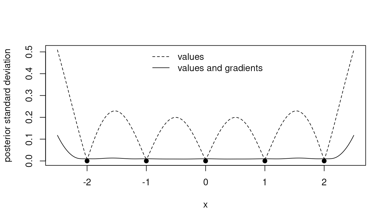
between <- abs(grid - round(grid)) > 0.4 & abs(grid) < 2
c(
  values = max(before$latent_sd[between]),
  values_and_gradients = max(after$latent_sd[between])
)
#>               values values_and_gradients 
#>           0.22944994           0.01335559

The posterior gradient is constrained too. At the observed points it reproduces \cos x up to the noise:

predict_gradient_gp(with_gradients, x_observed)$mean[, 1] - cos(x_observed)
#> [1] 1.012559e-05 2.584515e-05 2.948141e-05 2.584515e-05 1.012559e-05

Derivative blocks scale with 1 / \ell^2, so they can be conditioned differently from the values. gp_numerical_diagnostics() reports each observation type separately:

gp_numerical_diagnostics(with_gradients)$observation_types
#>            type observations covariance_scale reciprocal_condition_number
#> 1         value            5           1.0001                   0.1095987
#> 2 derivative x1            5           1.5626                   0.1157423

Verification

The tests check that conditioning on a derivative equals the limit h \to 0 of conditioning on difference quotients (f(x + h e_d) - f(x - h e_d)) / 2h, for the posterior mean, covariance, and log marginal likelihood, by Richardson extrapolation to 10^{-6}. They also check that the log-marginal-likelihood gradient, including the derivative blocks, matches central differences to 10^{-6} for single, ARD, periodic, product, sum, scaled, and column-restricted kernels, and that the hyperparameter derivatives of every kernel’s input derivatives match central differences.