Gaussian-Process Regression from First Principles • gaussianprocesses

Model

Let

f \sim \mathcal{GP}(m,k),

where m(x) is a mean function and k(x,x') is a positive semidefinite covariance kernel.

For training inputs

X = (x_1,\ldots,x_n)^\top

and observations

y_i = f(x_i) + \varepsilon_i, \qquad \varepsilon_i \sim \mathcal N(0,\sigma_i^2),

define

K_{ff} = K(X,X), \qquad \Sigma_\varepsilon = \operatorname{diag}(\sigma_1^2,\ldots,\sigma_n^2).

Then

y \sim \mathcal N\left( m(X), K_{ff}+\Sigma_\varepsilon \right).

The package represents the same objects explicitly:

Mathematics	Package object
m	`zero_mean()`, `constant_mean()`
k	kernel specification such as `rbf_kernel()`
K(X,X)	`evaluate_kernel(kernel, X)`
\Sigma_\varepsilon	`noise_variance` in `fit_gp()`
fitted conditional model	`fit_gp()`

A scalar noise_variance gives the usual homoscedastic model. A vector gives one known observation variance per training point.

Conditioning

At prediction inputs X_*, define

K_{f*} = K(X,X_*), \qquad K_{**} = K(X_*,X_*).

Write

C = K_{ff}+\Sigma_\varepsilon.

The posterior latent mean is

\mu_* = m(X_*) + K_{*f}C^{-1}\left(y-m(X)\right),

and the latent covariance is

\Sigma_* = K_{**} - K_{*f}C^{-1}K_{f*}.

The implementation never forms C^{-1}. It computes a Cholesky factorization

C = R^\top R

and solves triangular systems.

The stored vector

\alpha = C^{-1}\left(y-m(X)\right)

corresponds directly to model$alpha.

Minimal reproducible fit

x <- c(-1.5, -0.5, 0.5, 1.5)
y <- c(0.9, -0.1, 0.2, 1.0)

kernel <- rbf_kernel(
  variance = 1.2,
  length_scale = 0.7
)

model <- fit_gp(
  x,
  y,
  kernel = kernel,
  noise_variance = 0.05
)

model
#> Exact Gaussian-process regression model
#>   observations: 4
#>   input dimensions: 1
#>   mean: ZeroMean()
#>   noise structure: homoscedastic
#>   noise variance: 0.05
#>   numerical jitter: 0
#>   kernel:
#>     RBF(variance=1.2, length_scale=0.7)

The fitted object stores the Cholesky factor R and the vector \alpha. The covariance matrices are not stored, because the kernel recomputes them exactly, and R^\top R reproduces C plus any numerical jitter (here none):

K <- evaluate_kernel(model$kernel, model$x)
C <- K + diag(model$training_noise_variance)
C
#>              [,1]       [,2]       [,3]         [,4]
#> [1,] 1.2500000000 0.43253735 0.02025586 0.0001232431
#> [2,] 0.4325373463 1.25000000 0.43253735 0.0202558610
#> [3,] 0.0202558610 0.43253735 1.25000000 0.4325373463
#> [4,] 0.0001232431 0.02025586 0.43253735 1.2500000000

model$cholesky
#>          [,1]      [,2]       [,3]        [,4]
#> [1,] 1.118034 0.3868732 0.01811739 0.000110232
#> [2,] 0.000000 1.0489658 0.40566454 0.019269662
#> [3,] 0.000000 0.0000000 1.04168519 0.407722346
#> [4,] 0.000000 0.0000000 0.00000000 1.040860777
all.equal(crossprod(model$cholesky), C + diag(model$jitter, nrow(C)))
#> [1] TRUE

model$alpha
#> [1]  0.854689487 -0.389576989  0.002244874  0.805451913

?gaussianprocesses_model describes every field of a fitted model, how models are versioned, and how to save them.

Posterior prediction

x_new <- seq(-2, 2, length.out = 80)

prediction <- predict_gp(
  model,
  x_new,
  interval_level = 0.95
)

head(
  data.frame(
    x = x_new,
    mean = prediction$mean,
    latent_sd = prediction$latent_sd,
    observation_sd = prediction$observation_sd
  )
)
#>           x      mean latent_sd observation_sd
#> 1 -2.000000 0.7476407 0.6836559      0.7192950
#> 2 -1.949367 0.7798487 0.6305943      0.6690659
#> 3 -1.898734 0.8085496 0.5750144      0.6169615
#> 4 -1.848101 0.8331786 0.5176677      0.5638970
#> 5 -1.797468 0.8532069 0.4595633      0.5110758
#> 6 -1.746835 0.8681562 0.4020650      0.4600611

The package reports two uncertainty layers.

The latent variance is

\operatorname{Var}\left[f(x_*)\mid y\right].

The observation variance is

\operatorname{Var}\left[y_*\mid y\right] = \operatorname{Var}\left[f(x_*)\mid y\right] + \sigma_*^2.

They are deliberately not conflated.

plot(
  x_new,
  prediction$mean,
  type = "l",
  xlab = "x",
  ylab = "response",
  ylim = range(prediction$prediction_interval)
)
polygon(
  c(x_new, rev(x_new)),
  c(
    prediction$prediction_interval[, "lower"],
    rev(prediction$prediction_interval[, "upper"])
  ),
  border = NA,
  density = 15
)
lines(x_new, prediction$mean)
points(x, y)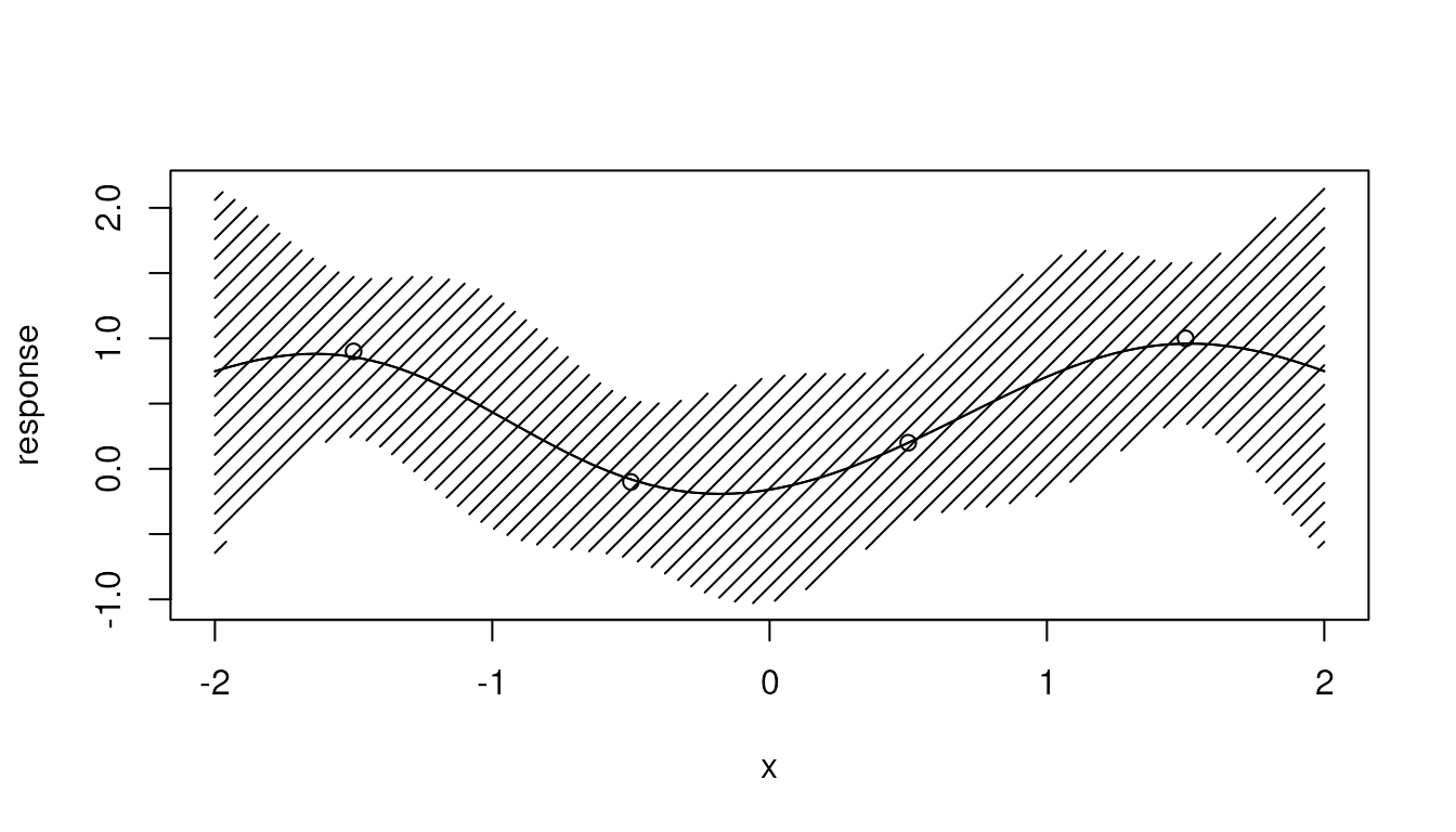

Posterior mean of the fitted Gaussian process for x from -2 to 2, with a hatched 95% prediction band and the four training observations as points.

Function draws

A mean and an interval summarize each input separately. Draws show whole functions, including how values at nearby inputs move together.

A draw from \mathcal N(\mu, \Sigma) is

f = \mu + R^\top z, \qquad \Sigma = R^\top R, \qquad z \sim \mathcal N(0, I),

where R is the Cholesky factor of the covariance. No inverse is needed. For the prior, \mu = m(X_*) and \Sigma = K_{**}. For the latent posterior, \mu and \Sigma are the posterior mean and covariance from predict_gp(). Closely spaced inputs make \Sigma numerically singular, so the factorization uses the package’s jitter policy and reports the jitter.

prior_draws <- sample_gp_prior(x_new, kernel, n_draws = 5, seed = 1)
posterior_draws <- sample_gp_posterior(model, x_new, n_draws = 5, seed = 1)

old_par <- par(mfrow = c(1, 2), mar = c(4, 4, 2, 1))
matplot(
  x_new, prior_draws$latent,
  type = "l", lty = 1, col = "grey40",
  xlab = "x", ylab = "f(x)", main = "Prior draws"
)
matplot(
  x_new, posterior_draws$latent,
  type = "l", lty = 1, col = "grey40",
  xlab = "x", ylab = "f(x)", main = "Posterior draws"
)
points(x, y, pch = 19)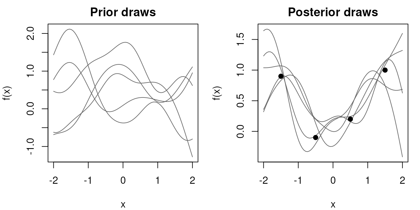

Two panels. Left: five smooth prior function draws spread around zero across x from -2 to 2. Right: five posterior function draws that pass close to the four training observations and fan out between and beyond them.

par(old_par)

The posterior draws agree near the observations and spread apart away from them, which is what the pointwise intervals summarize.

The 80 closely spaced inputs make both covariance matrices numerically singular, so both factorizations needed a small jitter:

c(prior = prior_draws$jitter, posterior = posterior_draws$jitter)
#>        prior    posterior 
#> 1.200000e-10 1.281765e-11

Latent draws are values of the function f. A future observation also includes noise, y_* = f_* + \varepsilon_*. With type = "observation", each noisy draw is generated from a latent draw plus independent noise, and both are returned:

noisy <- sample_gp_posterior(
  model,
  x_new,
  n_draws = 1,
  type = "observation",
  seed = 2
)

plot(
  x_new, noisy$observation[, 1],
  pch = 20, cex = 0.6, col = "grey50",
  xlab = "x", ylab = "response"
)
lines(x_new, noisy$latent[, 1])
points(x, y, pch = 19)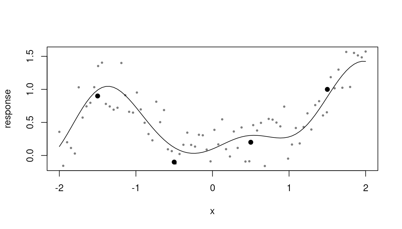

One latent posterior function draw as a line, with the corresponding noisy observation draws as small points scattered around it, and the training observations as larger points.

Over many draws, the latent draws reproduce the posterior covariance and the observation draws reproduce that covariance plus the noise variance:

many <- sample_gp_posterior(
  model,
  c(-1, 0.5),
  n_draws = 5000,
  type = "observation",
  seed = 3
)

round(
  rbind(
    latent_sample = apply(many$latent, 1, var),
    latent_theory = diag(many$latent_covariance),
    observation_sample = apply(many$observation, 1, var),
    observation_theory = diag(many$latent_covariance) +
      many$observation_noise_variance
  ),
  4
)
#>                      [,1]   [,2]
#> latent_sample      0.1578 0.0471
#> latent_theory      0.1553 0.0473
#> observation_sample 0.2085 0.0978
#> observation_theory 0.2053 0.0973

Known heteroscedastic observation variance

Exact conditioning also supports a known diagonal observation covariance:

known_noise <- c(0.02, 0.04, 0.08, 0.16)

heterogeneous_fit <- fit_gp(
  x,
  y,
  kernel = kernel,
  noise_variance = known_noise
)

heterogeneous_fit$training_noise_variance
#> [1] 0.02 0.04 0.08 0.16

For unknown input-dependent noise, see the package’s heteroscedastic GP approximation. The exact model above is still the underlying conditioning mechanism once a diagonal noise estimate has been supplied.