Multi-output Gaussian processes

Several outputs measured on the same inputs, such as related sensors or responses, are often correlated. A multi-output Gaussian process shares information between them, so an output can be predicted where it was not observed but the others were. This page sets out the coregionalization models of the package and compares one with independent Gaussian processes on a seeded study. The functions are experimental: they may change in a minor release.

Coregionalization

The intrinsic coregionalization model (ICM; Bonilla, Chai, and Williams, 2008) gives outputs p and q the covariance

\operatorname{cov}\bigl(f_p(x), f_q(x')\bigr) = B_{pq}\, k(x, x'), \qquad B = W W^\top + \operatorname{diag}(\kappa),

with an input kernel k, a P \times R matrix W, and positive \kappa, so B is positive semidefinite by construction. A sum of such terms with different input kernels is the linear model of coregionalization (LMC; Álvarez, Rosasco, and Lawrence, 2012). In the package, B is the kernel coregionalization_kernel() on a column that holds the output index, so an ICM is a product kernel and an LMC a sum of them; every fitting and prediction function then works unchanged.

gp_stack_outputs() turns inputs and one response column per output into that format. Missing values mark outputs that were not observed at an input, so each output can have its own inputs (heterotopic data):

x <- c(0, 1, 2, 3)
y <- cbind(c(1.0, NA, 0.4, 0.1), c(0.2, 0.3, NA, 0.5))
gp_stack_outputs(x, y)$x
#>        output
#> [1,] 0      1
#> [2,] 2      1
#> [3,] 3      1
#> [4,] 0      2
#> [5,] 1      2
#> [6,] 3      2

Two cautions:

• W is identified only up to rotation and sign, since W Q gives the same B for any orthogonal Q, and the scale of B trades off with the variance of the input kernel. coregionalization_matrix() reports B; its correlations cov2cor(B) are what can be interpreted.
• W = 0 is a stationary point of the likelihood, so an optimization started there stays there. initialize_coregionalization() starts W and \kappa from the empirical covariance between the outputs.

optimize_gp(noise_groups = ) estimates one noise variance per output.

A heterotopic study

Three outputs are built from two latent functions, u(x) = \sin x and v(x) = \cos 1.7x: f_1 = u, f_2 = 0.8u + 0.5v, and f_3 = -u + 0.4v, with noise standard deviations 0.1, 0.2, and 0.15. Each output is observed at 30 uniform random inputs on [0, 10], but output 1 is never observed in the gap 4 < x < 6.5, where the other two are. The question is how well output 1 is predicted in the gap.

The independent model is a Matérn-5/2 Gaussian process for output 1 alone. The ICM has rank 2, a Matérn-5/2 input kernel, a start from initialize_coregionalization(), and one noise variance per output. Both estimate their hyperparameters by maximum likelihood with two starts. Each replicate draws new inputs and noise; the error is the root mean square error of the predictive mean against f_1 at 20 points in the gap.

truth <- function(x) {
  u <- sin(x)
  v <- cos(1.7 * x)
  cbind(u, 0.8 * u + 0.5 * v, -u + 0.4 * v)
}
noise_sd <- c(0.1, 0.2, 0.15)
gap <- c(4, 6.5)
test_x <- seq(gap[1] + 0.1, gap[2] - 0.1, length.out = 20)

replicate_study <- function(seed, n = 30) {
  set.seed(seed)
  inputs <- lapply(1:3, function(p) sort(runif(n, 0, 10)))
  inputs[[1]] <- inputs[[1]][inputs[[1]] < gap[1] | inputs[[1]] > gap[2]]
  x <- sort(unique(unlist(inputs)))
  y <- matrix(NA_real_, length(x), 3)
  for (p in 1:3) {
    rows <- match(inputs[[p]], x)
    y[rows, p] <- truth(inputs[[p]])[, p] +
      rnorm(length(rows), sd = noise_sd[[p]])
  }
  stacked <- gp_stack_outputs(x, y)
  first <- stacked$output == 1

  independent <- optimize_gp(stacked$x[first, 1], stacked$y[first],
                             matern52_kernel(), noise_variance = 0.05,
                             n_starts = 2)
  start <- initialize_coregionalization(stacked$output, stacked$y,
                                        x = stacked$x[, 1], rank = 2)
  icm <- optimize_gp(
    stacked$x, stacked$y,
    product_kernel(select_dimensions(matern52_kernel(), 1),
                   select_dimensions(start, 2)),
    noise_variance = 0.05, noise_groups = stacked$output, n_starts = 2
  )

  separate <- predict_gp(independent, test_x)
  joint <- predict_gp(
    icm, gp_stack_outputs(test_x, outputs = 1)$x,
    observation_noise_variance =
      icm$optimization$optimized_parameters[["noise_variance[1]"]]
  )
  covered <- function(prediction) {
    mean(abs(prediction$mean - truth(test_x)[, 1]) <=
           qnorm(0.975) * prediction$latent_sd)
  }

  list(
    summary = c(
      rmse_independent = sqrt(mean((separate$mean - truth(test_x)[, 1])^2)),
      rmse_icm = sqrt(mean((joint$mean - truth(test_x)[, 1])^2)),
      coverage_independent = covered(separate),
      coverage_icm = covered(joint)
    ),
    correlation = cov2cor(coregionalization_matrix(icm$kernel)[[1]]),
    data = stacked,
    separate = separate,
    joint = joint
  )
}

replicates <- lapply(1:15, replicate_study)
results <- t(vapply(replicates, `[[`, numeric(4), "summary"))

Mean over 15 replicates, with its Monte Carlo standard error in parentheses.

Model	RMSE in the gap	Coverage of 95% intervals
independent GP for output 1	0.263 (0.043)	1.000 (0.000)
ICM, rank 2	0.090 (0.010)	0.910 (0.053)

Over 15 replicates the ICM reduced the error in the gap by 0.173 (0.043) (paired difference, with its Monte Carlo standard error), and was more accurate in 14 of them. Outputs 2 and 3 are observed in the gap and share u with output 1, so the ICM can reconstruct f_1 there, while the independent model can only interpolate across the gap.

The correlations between the latent functions over [0, 10], and those the ICM estimated in the first replicate:

grid <- seq(0, 10, length.out = 2001)
round(cor(truth(grid)), 2)
#>       u            
#> u  1.00  0.84 -0.92
#>    0.84  1.00 -0.55
#>   -0.92 -0.55  1.00
round(replicates[[1]]$correlation, 2)
#>       [,1] [,2]  [,3]
#> [1,]  1.00 0.51 -0.78
#> [2,]  0.51 1.00  0.14
#> [3,] -0.78 0.14  1.00

The estimates have the right signs between output 1 and the other two, which is what predicting output 1 relies on, but they are weaker, and the correlation between outputs 2 and 3 is estimated poorly. One B has to describe two latent functions with different length scales, which is the misspecification discussed below.

first <- replicates[[1]]
observed <- first$data$output == 1
plot(first$data$x[observed, 1], first$data$y[observed], pch = 16,
     cex = 0.7, xlim = c(2, 8.5), ylim = c(-2, 2), xlab = "x",
     ylab = "output 1")
rect(gap[1], -3, gap[2], 3, col = grDevices::adjustcolor("grey", 0.2),
     border = NA)
curve(truth(x)[, 1], add = TRUE, lty = 3)
for (model in c("separate", "joint")) {
  prediction <- first[[model]]
  colour <- if (model == "joint") "steelblue" else "darkorange"
  lines(test_x, prediction$mean, col = colour, lwd = 2)
  matlines(test_x, prediction$latent_interval, col = colour, lty = 2)
}
legend("topright", c("truth", "independent GP", "ICM"),
       col = c("black", "darkorange", "steelblue"), lty = c(3, 1, 1),
       bty = "n")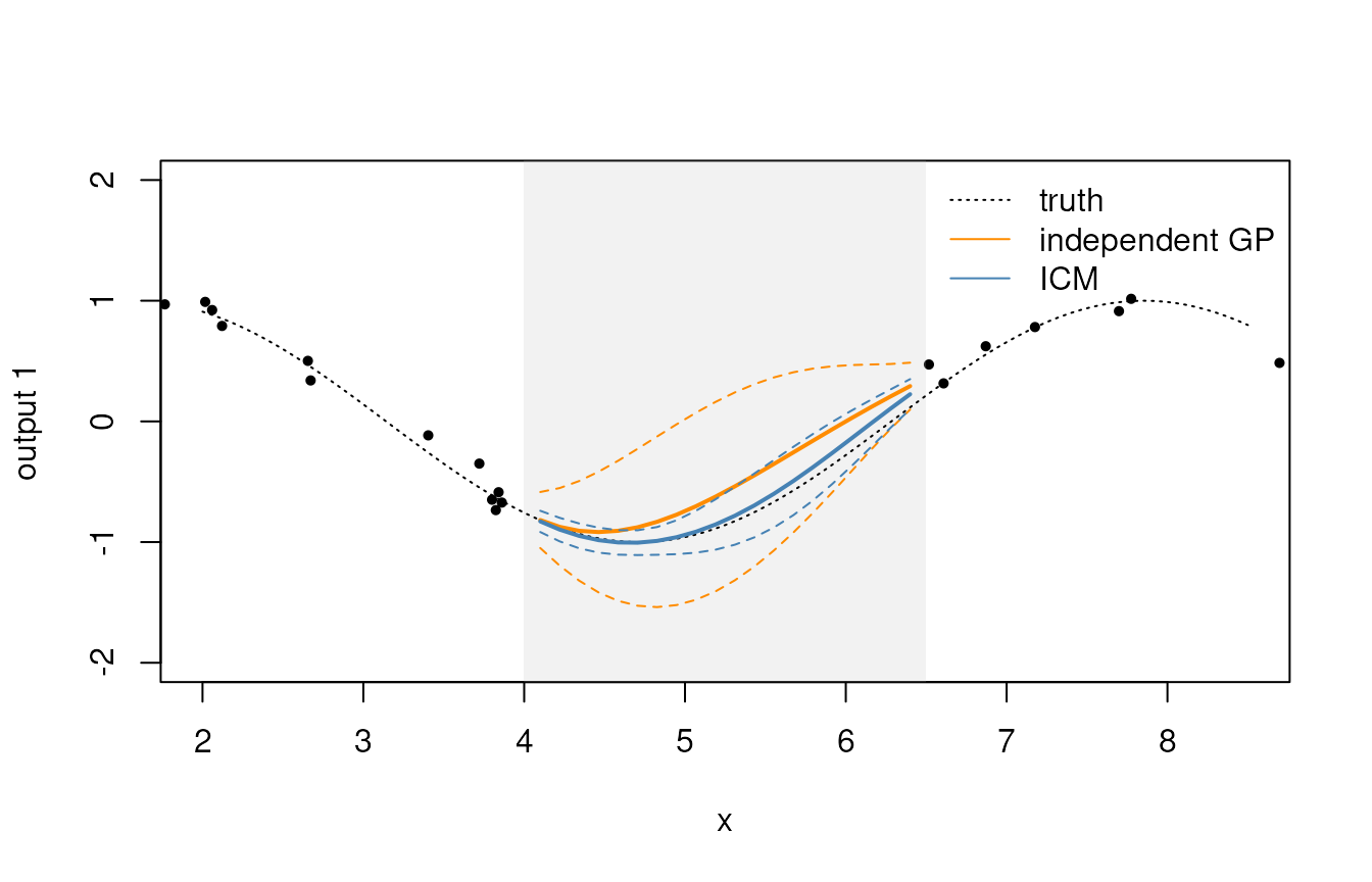

The intervals tell a less tidy story. The independent model’s intervals are wide in the gap and covered the truth at every test point. The ICM’s are much narrower, and their coverage, 0.910 (0.053), is below the nominal 95%: in some replicates the ICM is confidently wrong over part of the gap. The model is misspecified: the two latent functions have different length scales, but an ICM gives all outputs one input kernel. An LMC with one ICM term per latent function matches the construction better; this page does not test it. Either way, a smaller error does not make the intervals calibrated, and they should be checked, for example with gp_scores() on held-out data.

References

Álvarez, M. A., Rosasco, L., and Lawrence, N. D. (2012). Kernels for vector-valued functions: a review. Foundations and Trends in Machine Learning, 4(3), 195–266.

Bonilla, E. V., Chai, K. M. A., and Williams, C. K. I. (2008). Multi-task Gaussian process prediction. Advances in Neural Information Processing Systems, 20.