Research note: count data with latent Gaussian processes
Source:vignettes/articles/gp-counts.Rmd
gp-counts.RmdA Poisson Gaussian-process model lets the rate of a count vary
smoothly with the inputs:
y_i \sim \mathrm{Poisson}\bigl(E_i\, e^{f(x_i)}\bigr), \qquad
f \sim \mathcal{GP}(\beta_0, k),
where E_i is a known exposure,
such as a population or an observation period, entering as the offset
\log E_i, and \beta_0 is a mean log rate.
fit_latent_gp() and optimize_latent_gp() fit
it with poisson_likelihood() and the Laplace approximation.
This note analyses a classic count series and checks the predictive
distributions in a simulation from a known log-intensity process.
The discoveries series
datasets::discoveries counts the “great” inventions and
scientific discoveries in each year from 1860 to 1959. A constant-rate
Poisson model would give a variance equal to the mean; the series has
mean 3.1 and variance 5.08, more variable than that.
counts <- as.numeric(discoveries)
years <- as.numeric(time(discoveries))
time_index <- gp_time_index(years)

model <- optimize_latent_gp(
  time_index,
  counts,
  matern52_kernel(variance = 0.2, length_scale = 10),
  poisson_likelihood(),
  mean = constant_mean(estimate_coefficients()),
  n_starts = 3
)
model
#> Latent Gaussian-process model (Laplace approximation)
#>   observations: 100
#>   input dimensions: 1
#>   likelihood: PoissonLikelihood(link=log)
#>   mean: ConstantMean(estimated by ML)
#>   mean coefficients: intercept=1.03679
#>   Newton iterations: 5 (converged)
#>   approximate log marginal likelihood: -204.3895
#>   numerical jitter: 0
#>   optimization: converged (L-BFGS-B, analytical gradient)
#>   kernel:
#>     Matern-5/2(variance=0.165919, length_scale=3.41995)
exp(coef(model))
#> intercept
#>  2.820158
gp_time_index() measures time in years since 1860, so
the length scale is in years. The mean level, estimated jointly with the
kernel parameters, is a rate of 2.82 discoveries a year; the latent
process varies around it with a standard deviation of 0.41 on the log
scale over about 3.4 years.
prediction <- predict_latent_gp(model, time_index, interval_level = 0.9)

plot(years, counts, pch = 19, cex = 0.6, ylim = c(0, 16.5),
     xlab = "year", ylab = "discoveries", yaxt = "n")
axis(2, at = seq(0, 12, by = 2))
segments(years, prediction$prediction_interval[, "lower"],
         years, prediction$prediction_interval[, "upper"], col = "grey80",
         lwd = 3)
points(years, counts, pch = 19, cex = 0.6)
polygon(c(years, rev(years)),
        c(prediction$rate_interval[, "lower"],
          rev(prediction$rate_interval[, "upper"])),
        col = adjustcolor("#0072B2", 0.25), border = NA)
lines(years, prediction$response_mean, col = "#0072B2", lwd = 2)
legend("top", c("counts", "posterior mean rate", "90% interval of the rate",
                "90% prediction interval of a count"),
       pch = c(19, NA, 15, 15), lty = c(NA, 1, NA, NA), lwd = c(NA, 2, NA, NA),
       col = c("black", "#0072B2", adjustcolor("#0072B2", 0.25), "grey80"),
       bty = "n", cex = 0.8, ncol = 2)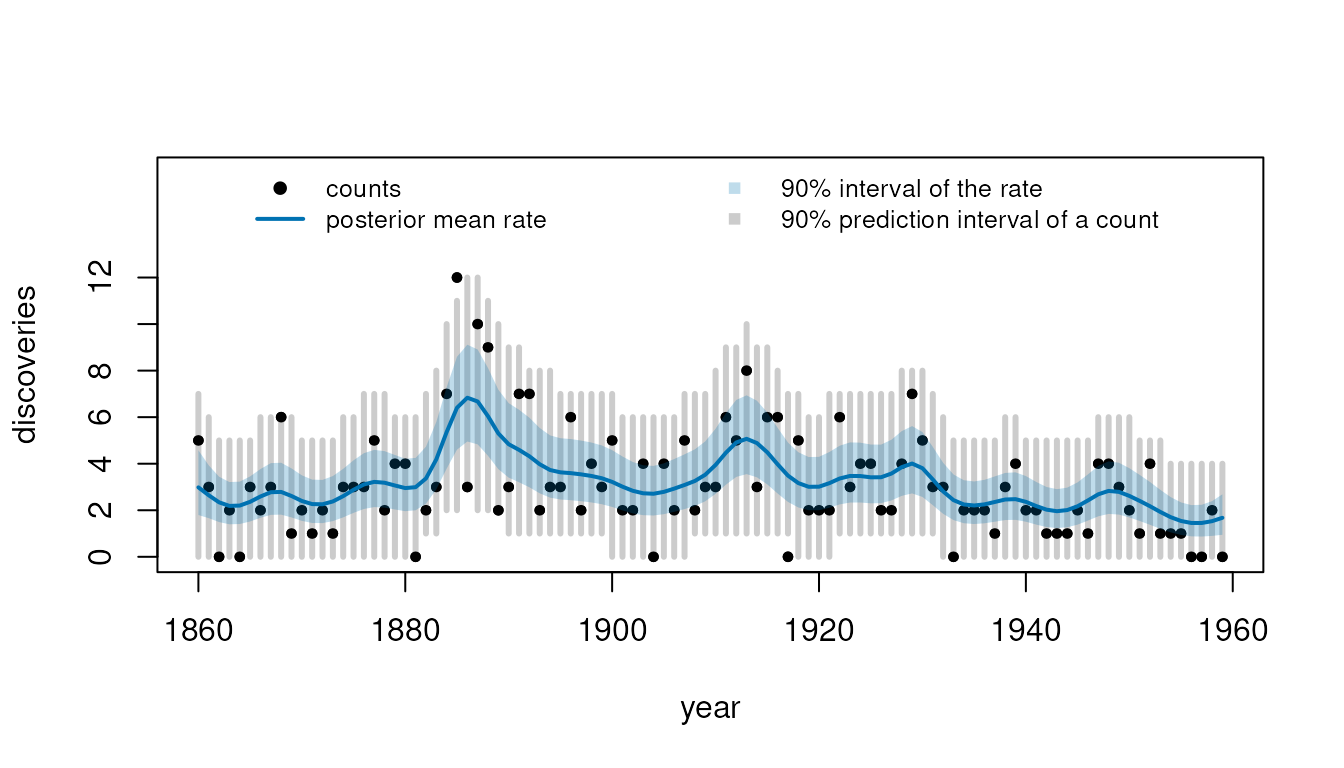
Two kinds of uncertainty appear. The rate \lambda(t) = e^{f(t)} is lognormal under the
Laplace approximation, so its interval rate_interval is
e^{\mu \pm z \sigma} exactly. A new
count adds Poisson variation: its predictive distribution is a
Poisson–lognormal mixture, and prediction_interval gives
its equal-tailed quantiles. Counts are discrete, so these intervals
cover at least their level, and usually more.
Checking the model on held-out years
Fitting on the even years and predicting the odd ones checks the
predictive distributions on counts the model has not seen.
gp_holdout_scores() returns count scores for Poisson
models: the log score, the Dawid–Sebastiani score, the coverage of the
count intervals, a dispersion check, and randomized PIT values.
even <- years %% 2 == 0
training_fit <- optimize_latent_gp(
  time_index[even],
  counts[even],
  matern52_kernel(variance = 0.2, length_scale = 10),
  poisson_likelihood(),
  mean = constant_mean(estimate_coefficients()),
  n_starts = 3
)
scores <- gp_holdout_scores(training_fit, time_index[!even], counts[!even],
                            seed = 1)
scores
#> Count scores for 50 observations
#>   log score (mean): -2.096
#>   Dawid-Sebastiani score (mean): 2.531
#>   dispersion: 1.287 (about 1 if the predictive variance is right)
#>   randomized PIT mean and variance: 0.4673, 0.09176 (0.5 and 0.0833 if calibrated)
#>   coverage: 50% 60%, 80% 86%, 90% 90%, 95% 96%

# A constant rate, the mean of the training years, for comparison.
constant_rate <- mean(counts[even])
c(
  log_score = mean(dpois(counts[!even], constant_rate, log = TRUE)),
  dispersion = mean((counts[!even] - constant_rate)^2 / constant_rate)
)
#>  log_score dispersion
#>  -2.276325   1.956306
The time-varying rate predicts the held-out years better than a constant rate, by 0.18 in mean log score, and explains most of the extra variability: the dispersion, the mean squared Pearson residual (y - m)^2 / s^2 of the predictive distribution, is 1.29 against 1.96 for the constant rate. With 50 held-out years its standard error is about 0.29, so the remaining excess over 1 is not clear evidence of overdispersion beyond the model.
Randomized PIT values u = F(y - 1) + v\, p(y), with v uniform, are uniform for calibrated count forecasts; the plain PIT F(y) of a discrete distribution is not.
hist(scores$pointwise$pit, breaks = seq(0, 1, by = 0.1), main = NULL,
     xlab = "randomized PIT", col = "grey85", border = "white")
abline(h = nrow(scores$pointwise) / 10, lty = 2)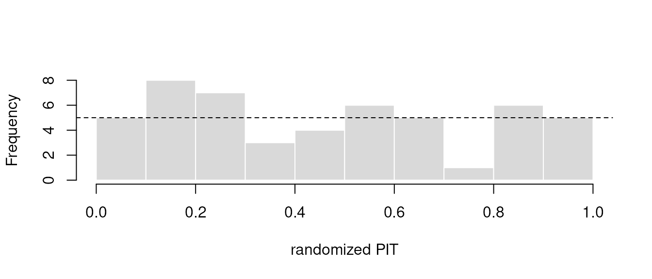
Exposure
When counts come from units of different size, the exposure enters as
an offset: exposure = population models a rate per person.
Doubling every exposure while lowering the mean log rate by \log 2 gives the same fit, and an estimated
mean level absorbs the shift exactly; the test suite checks both.
Predictions take the exposure of the new units, defaulting to 1.
Simulation study
The script below, inst/examples/gp-counts-study.R, draws
counts from a known log-intensity Gaussian process with random
exposures, fits each data set with the true hyperparameters and with
estimated ones, and checks the intervals and PIT values on 100 held-out
inputs. A last group of data sets multiplies each rate by independent
gamma noise, overdispersion that a Poisson model with a smooth rate
cannot describe. It is run as-is to produce this page.
# Coverage and calibration of Poisson Gaussian-process models on counts from
# a known log-intensity process.
#
# Each replicate draws a log intensity f from a Gaussian process with mean
# log(5) and an RBF kernel (variance 0.5, length scale 1.5) at 160 uniform
# inputs on [0, 10], exposures uniform on [0.5, 2], and counts
# y ~ Poisson(E exp(f)). The first 60 are for training, the other 100 for
# testing. The model is fitted with the true hyperparameters and mean
# ("known") and with hyperparameters and mean level estimated by
# optimize_latent_gp() ("estimated"). For each fit the script records, at
# the test inputs,
#   the coverage of the rate intervals E exp(mu -+ z sigma) of the true
#     rate E exp(f) at levels 0.8 and 0.95;
#   the coverage and mean width of the count prediction intervals;
#   the randomized PIT values of the test counts and their dispersion.
# A last set of replicates adds overdispersion, multiplying each rate by an
# independent gamma variable with mean 1 and variance 0.5, which the Poisson
# model does not describe.

library(gaussianprocesses)

n_replicates <- 150
n_overdispersed <- 40
n_training <- 60
n_test <- 100
levels <- c(0.8, 0.95)
kernel <- rbf_kernel(variance = 0.5, length_scale = 1.5)
log_level <- log(5)

simulate_counts <- function(overdispersion = 0) {
  x <- stats::runif(n_training + n_test, 0, 10)
  f <- log_level + drop(sample_gp_prior(x, kernel)$latent)
  exposure <- stats::runif(length(x), 0.5, 2)
  rate <- exposure * exp(f)

  if (overdispersion > 0) {
    rate <- rate * stats::rgamma(length(x), 1 / overdispersion,
                                 1 / overdispersion)
  }

  list(x = x, f = f, exposure = exposure, y = stats::rpois(length(x), rate))
}

# The rate intervals at both levels come from one prediction: they are the
# exponential of the latent intervals, scaled by the exposure.
evaluate <- function(model, data, test) {
  prediction <- predict_latent_gp(model, data$x[test],
                                  exposure = data$exposure[test])
  true_rate <- data$exposure[test] * exp(data$f[test])
  rate_coverage <- vapply(levels, function(level) {
    half_width <- stats::qnorm((1 + level) / 2) * prediction$latent_sd
    lower <- data$exposure[test] * exp(prediction$mean - half_width)
    upper <- data$exposure[test] * exp(prediction$mean + half_width)
    mean(true_rate >= lower & true_rate <= upper)
  }, numeric(1))
  scores <- gp_holdout_scores(model, data$x[test], data$y[test],
                              interval_levels = levels,
                              exposure = data$exposure[test])

  list(
    intervals = data.frame(
      level = levels,
      rate_coverage = rate_coverage,
      count_coverage = scores$calibration$coverage,
      count_width = scores$calibration$width
    ),
    pit = scores$pointwise$pit,
    dispersion = scores$summary[["dispersion"]]
  )
}

set.seed(20261008)
results <- list()
pit <- list()
dispersion <- list()
estimates <- matrix(NA_real_, n_replicates, 3,
                    dimnames = list(NULL, c("variance", "length_scale",
                                            "mean_level")))
training <- seq_len(n_training)
test <- n_training + seq_len(n_test)

for (replicate in seq_len(n_replicates + n_overdispersed)) {
  overdispersed <- replicate > n_replicates
  data <- simulate_counts(if (overdispersed) 0.5 else 0)
  fits <- list(known = fit_latent_gp(
    data$x[training], data$y[training], kernel, poisson_likelihood(),
    mean = constant_mean(log_level), exposure = data$exposure[training]
  ))

  if (!overdispersed) {
    fits$estimated <- optimize_latent_gp(
      data$x[training], data$y[training], rbf_kernel(), poisson_likelihood(),
      mean = constant_mean(estimate_coefficients()),
      exposure = data$exposure[training], n_starts = 1
    )
    estimates[replicate, ] <- c(
      kernel_parameters(fits$estimated$kernel, flatten = TRUE),
      coef(fits$estimated)
    )
  }

  for (fit in names(fits)) {
    label <- if (overdispersed) "overdispersed" else fit
    evaluation <- evaluate(fits[[fit]], data, test)
    results[[length(results) + 1L]] <- cbind(
      replicate = replicate,
      fit = label,
      evaluation$intervals
    )
    pit[[label]] <- rbind(pit[[label]], evaluation$pit)
    dispersion[[label]] <- c(dispersion[[label]], evaluation$dispersion)
  }
}

results <- do.call(rbind, results)

# Coverage averaged over replicates, with Monte Carlo standard errors from
# the spread of the per-replicate coverages.
coverage <- do.call(rbind, lapply(
  split(results, list(results$fit, results$level), drop = TRUE),
  function(rows) {
    data.frame(
      fit = rows$fit[1],
      level = rows$level[1],
      rate_coverage = mean(rows$rate_coverage),
      rate_coverage_se = stats::sd(rows$rate_coverage) / sqrt(nrow(rows)),
      count_coverage = mean(rows$count_coverage),
      count_coverage_se = stats::sd(rows$count_coverage) / sqrt(nrow(rows)),
      count_width = mean(rows$count_width)
    )
  }
))
coverage <- coverage[order(coverage$fit, coverage$level), ]
rownames(coverage) <- NULL

# PIT values of one data set share its latent function, so they are not
# independent. The Kolmogorov-Smirnov test uses the first test count of each
# data set, which are; the mean and variance pool all test counts.
calibration <- data.frame(
  fit = names(pit),
  pit_mean = vapply(pit, mean, numeric(1)),
  pit_variance = vapply(pit, function(values) stats::var(c(values)),
                        numeric(1)),
  ks_p_value = vapply(
    pit,
    function(values) {
      suppressWarnings(stats::ks.test(values[, 1], "punif"))$p.value
    },
    numeric(1)
  ),
  dispersion = vapply(dispersion, mean, numeric(1))
)
rownames(calibration) <- NULL

print(coverage, digits = 3)
#>             fit level rate_coverage rate_coverage_se count_coverage
#> 1     estimated  0.80         0.743          0.01335          0.866
#> 2     estimated  0.95         0.911          0.00863          0.969
#> 3         known  0.80         0.792          0.01082          0.871
#> 4         known  0.95         0.948          0.00565          0.972
#> 5 overdispersed  0.80         0.521          0.02582          0.560
#> 6 overdispersed  0.95         0.710          0.02631          0.739
#>   count_coverage_se count_width
#> 1           0.00296        7.04
#> 2           0.00170       10.71
#> 3           0.00270        7.05
#> 4           0.00145       10.73
#> 5           0.01399        7.08
#> 6           0.01362       10.75
print(calibration, digits = 3)
#>             fit pit_mean pit_variance ks_p_value dispersion
#> 1         known    0.494       0.0836    0.75767      0.994
#> 2     estimated    0.495       0.0843    0.78750      1.026
#> 3 overdispersed    0.440       0.1433    0.00395      4.620
print(round(apply(estimates, 2, stats::median), 2))
#>     variance length_scale   mean_level
#>         0.32         1.34         1.54
Rate intervals. With the true hyperparameters the 80% and 95% rate intervals cover the true rate in 79.2% (Monte Carlo standard error 1.1) and 94.8% (0.6) of the test inputs, as they should. With estimated hyperparameters they cover 74.3% and 91.1%: the intervals treat the estimates as known, and with 60 training counts the signal variance is often underestimated (median estimate 0.32 against the true 0.5), which makes them too narrow.
Count intervals. The 80% and 95% count intervals cover 87.1% and 97.2% of the test counts with the true hyperparameters: more than their level, because the quantiles of a discrete distribution include the probability of their end points. With counts around five, that excess is several percentage points.
Randomized PIT. Pooled over all test counts, the randomized PIT values of the correctly specified model have mean 0.494 and variance 0.0836 (0.5 and 1/12 for uniform values). The PIT values of one data set share its latent function and are not independent, so the Kolmogorov–Smirnov test uses the first test count of each data set: its p-value is 0.76 with the true hyperparameters and 0.79 with estimated ones.
Overdispersion. On the overdispersed counts the dispersion is 4.6 instead of about 0.99, the PIT variance rises to 0.14 (too many values near 0 and 1), and the 95% count intervals cover only 73.9% of the counts. The dispersion check is the quickest sign that a Poisson model with a smooth rate is not enough.