Validation: independent references and reproductions
Source:vignettes/articles/validation.Rmd
validation.RmdEvery inference method in the package is checked against an independent computation of the same quantity. This page runs those checks while it is built and reports what they found, then reproduces three analyses on data that ship with R.
How the methods are checked
A reference compares one quantity computed by the package with one of three kinds of independent computation:
- implementation: another R package that computes the same model, such as DiceKriging, kernlab, nlme, or gplite, or LAPACK through base R;
- brute force: the defining formula evaluated directly, with dense matrices, refits, numerical integration, numerical differentiation, or a general-purpose optimizer;
- closed form: a formula the package does not use to compute the quantity, such as the exact Gaussian process that an approximation reduces to.
The references are defined in
inst/validation/references.R, installed as
system.file("validation", "references.R", package = "gaussianprocesses").
The test suite runs each one and fails if its discrepancy exceeds its
tolerance. A test also checks that every exported function belongs to a
method with at least one reference, or is listed as performing no
inference. References that need a suggested package are skipped when it
is not installed.
Unless a reference says otherwise, the discrepancy is the largest absolute difference divided by the largest absolute reference value. Tolerances depend on what limits the agreement:
- 1e-10 where both sides are exact up to rounding;
- 1e-6 for first and 1e-4 for second finite differences;
- 1e-7 for numerical integration against the package’s quadrature;
- 1e-6 in the log likelihood for two optimizers’ maxima;
- the convergence of iterative references;
- five Monte Carlo standard errors for sampling.
Except for sampling, each tolerance is at least 30 times the discrepancy observed with the recorded versions of the reference packages.
Reference table
37 of the 37 references pass on this build. The package versions are those installed for this build; the tolerances were set with the recorded versions.
| Method | Quantity | Reference | Type | Tolerance | Discrepancy | Status |
|---|---|---|---|---|---|---|
| Exact regression | posterior mean and covariance at 25 inputs; ARD RBF kernel, known per-observation noise, fixed constant mean | simple kriging with DiceKriging::km() and predict(type = “SK”); DiceKriging 1.6.1 (recorded 1.6.1) | implementation | 1.0e-10 | 6.0e-15 | pass |
| posterior mean and variance at 25 inputs; RBF kernel, known noise, zero mean | kernlab::gausspr() with the rbfdot kernel; kernlab 0.9.33 (recorded 0.9-33) | implementation | 1.0e-10 | 1.5e-14 | pass | |
| posterior mean and covariance at 25 inputs; composite ARD kernel on two inputs, per-observation noise, fixed linear mean | Gaussian conditioning with dense matrices and solve() | closed form | 1.0e-10 | 4.6e-15 | pass | |
| Marginal likelihood and gradient | log marginal likelihood; composite ARD kernel, per-observation noise, fixed linear mean (relative error) | the Gaussian log density with determinant() and solve() | closed form | 1.0e-10 | 1.8e-16 | pass |
| gradient in the log kernel parameters and log noise variance; sum of RBF, periodic x RBF, and rational quadratic kernels | Richardson-extrapolated central differences of log_marginal_likelihood() | brute force | 1.0e-06 | 1.8e-08 | pass | |
| Hyperparameter optimization | maximized profile log likelihood (absolute difference); RBF kernel with estimated variance, length scale, noise, and constant mean | maximum likelihood with DiceKriging::km(nugget.estim = TRUE); DiceKriging 1.6.1 (recorded 1.6.1) | implementation | 1.0e-06 | 2.1e-11 | pass |
| maximized log marginal likelihood (absolute difference); Matern-5/2 kernel with estimated variance, length scale, and noise | stats::optim() (BFGS, numerical gradients, three starts) on the dense log density | brute force | 1.0e-06 | 4.4e-12 | pass | |
| Mean coefficients | maximum-likelihood and REML log likelihoods and coefficients of a linear mean; Gaussian correlation with a nugget | generalized least squares with nlme::gls() and corGaus(fixed = TRUE); nlme 3.1.169 (recorded 3.1-168) | implementation | 1.0e-10 | 2.5e-14 | pass |
| generalized least-squares coefficients, concentrated log likelihood, and universal-kriging mean and covariance (vague coefficient prior) | DiceKriging::km() with a linear trend, logLikFun(), and predict(type = “UK”); DiceKriging 1.6.1 (recorded 1.6.1) | implementation | 1.0e-10 | 4.9e-15 | pass | |
| posterior mean, covariance, and log marginal likelihood with a Gaussian prior on the coefficients of a quadratic mean | the exact GP with covariance k(x, x’) + h(x)’ B h(x’) and mean h(x)’ b, by dense conditioning | closed form | 1.0e-10 | 2.5e-12 | pass | |
| Leave-one-out prediction | leave-one-out predictive means and variances of all 30 observations, with marginalized linear-mean coefficients (vague prior), which each refit re-estimates | 30 refits, each without one observation, predicting it with fit_gp() and predict_gp() | brute force | 1.0e-10 | 1.5e-15 | pass |
| Derivative observations and gradient prediction | posterior mean and covariance of function values given 12 values and 6 derivative observations; RBF + Matern-5/2 kernel | dense conditioning on a joint covariance built from central differences of evaluate_kernel() (step 1e-4) | brute force | 1.0e-06 | 8.7e-09 | pass |
| posterior mean of the gradient at 25 inputs on two dimensions; ARD Matern-5/2 kernel | Richardson-extrapolated central differences of the posterior mean from predict_gp() | brute force | 1.0e-06 | 4.8e-10 | pass | |
| Heteroscedastic regression | estimated noise variances (largest difference of log variances): the documented update applied to the returned estimate reproduces it | one step of the update recomputed with leave-one-out refits and dense conditioning of the log-noise GP | brute force | 1.0e-08 | 7.4e-11 | pass |
| Sparse approximations (FITC and VFE) | FITC log marginal likelihood (relative error), predictive mean, and covariance; 60 inputs, 9 inducing points | the FITC density N(y; 0, Q + diag(K - Q) + sigma^2 I) and predictive equations with dense matrices | closed form | 1.0e-10 | 2.3e-15 | pass |
| VFE bound (relative error), predictive mean, and covariance; 60 inputs, 9 inducing points | Titsias’s bound log N(y; 0, Q + sigma^2 I) - tr(K - Q) / (2 sigma^2) and the predictive equations with dense matrices | closed form | 1.0e-10 | 9.0e-16 | pass | |
| FITC and VFE log marginal likelihoods (relative error) and predictions when every input is an inducing point | the exact GP, to which both approximations reduce when Z = X | closed form | 1.0e-10 | 7.2e-15 | pass | |
| gradient of the VFE bound and the FITC objective in the log hyperparameters and the 6 x 2 inducing inputs | Richardson-extrapolated central differences of the objective, refitting with fit_sparse_gp() | brute force | 1.0e-06 | 3.2e-12 | pass | |
| the first 10 points chosen by greedy variance selection (number of differences) | the pivot order of LAPACK’s pivoted Cholesky decomposition, chol(pivot = TRUE) | implementation | 0 | 0 | pass | |
| State-space inference | log marginal likelihood (relative error), posterior means, and variances at 25 inputs; Matern-5/2 + scaled Matern-1/2 kernel on 200 irregular inputs with ties | the exact GP with dense matrices (fit_gp() and predict_gp()) | closed form | 1.0e-10 | 1.6e-14 | pass |
| Multi-output models | log marginal likelihood (relative error), posterior means, and covariances of three heterotopic outputs with W = 0 and kappa = 1 | three independent exact GPs, one per output, which the model equals in that case | closed form | 1.0e-10 | 1.0e-15 | pass |
| gradient of the log marginal likelihood in W, log kappa, the input kernel, and one log noise variance per output | Richardson-extrapolated central differences of log_marginal_likelihood(), refitting with fit_gp() | brute force | 1.0e-06 | 7.8e-12 | pass | |
| Laplace approximation | posterior mode, approximate log marginal likelihood (relative error), and latent predictive means and variances (absolute differences); logit and probit links | gplite with approx_laplace() and the same kernel and jitter; gplite 0.13.0 (recorded 0.13.0) | implementation | 1.0e-05 | 2.4e-07 | pass |
| posterior mode, approximate log marginal likelihood (relative error), and latent predictive means and variances (absolute differences); Poisson counts with exposure | gplite with approx_laplace() and an offset; gplite 0.13.0 (recorded 0.13.0) | implementation | 1.0e-05 | 5.7e-08 | pass | |
| log marginal likelihood (relative error), latent predictive means, and variances with a Gaussian likelihood | the exact GP, which the Laplace approximation equals for Gaussian observations | closed form | 1.0e-10 | 4.7e-15 | pass | |
| gradient of the approximate log marginal likelihood in the log kernel parameters; Bernoulli (logit) and Poisson likelihoods | Richardson-extrapolated central differences of the approximate log marginal likelihood, refitting with fit_latent_gp() | brute force | 1.0e-06 | 4.2e-12 | pass | |
| class probabilities (logit and probit links) and Poisson-lognormal probabilities, distribution function, and predictive mean (largest absolute difference) | stats::integrate() of the likelihood against the Gaussian latent predictive density | brute force | 1.0e-07 | 2.8e-10 | pass | |
| Posterior and prior sampling | sample means, variances, and correlations of 20 000 posterior and prior draws at 8 inputs (largest deviation in Monte Carlo standard errors) | the Gaussian posterior and prior moments from predict_gp() and evaluate_kernel() | closed form | 5.0e+00 | 2.7e+00 | pass |
| Hyperparameter uncertainty | observed information matrix of the log hyperparameters at the maximum | second-order central differences of log_marginal_likelihood() (step 1e-3) | brute force | 1.0e-04 | 8.0e-07 | pass |
| profile log likelihood of the length scale at 5 values (absolute difference) | stats::optim() (BFGS, numerical gradients) over the other log parameters of the dense log density | brute force | 1.0e-06 | 1.8e-13 | pass | |
| Predictive scores | pointwise CRPS and log scores of Gaussian predictions | stats::integrate() of (F(z) - 1{z >= y})^2 over z, and stats::dnorm() | brute force | 1.0e-10 | 4.4e-16 | pass |
| log loss, Brier score, and ROC AUC of 200 probability forecasts | direct formulas and the AUC as the fraction of correctly ordered positive-negative pairs | brute force | 1.0e-10 | 0 | pass | |
| pointwise log scores and predictive means and variances of Poisson-lognormal count forecasts (largest absolute difference) | stats::integrate() of the Poisson probabilities and moments against the latent predictive density | brute force | 1.0e-10 | 5.3e-15 | pass | |
| rolling-origin forecasts and forecast metrics (RMSE, coverage, log predictive density) | expanding-window refits with fit_gp() and predict_gp(), and the metrics computed directly | brute force | 1.0e-10 | 2.7e-15 | pass | |
| Kernels | covariance matrices of the RBF, Matern-1/2 (exponential), and linear kernels on 20 three-dimensional inputs | kernlab::kernelMatrix() with rbfdot, laplacedot, and vanilladot; kernlab 0.9.33 (recorded 0.9-33) | implementation | 1.0e-08 | 2.4e-10 | pass |
| derivatives of covariance matrices in every log parameter: rational quadratic x periodic, changepoint, and spectral-mixture kernels | Richardson-extrapolated central differences of evaluate_kernel() | brute force | 1.0e-06 | 1.5e-10 | pass | |
| spectral-mixture covariance at 30 lags | the Fourier integral of its spectral density, a mixture of Gaussians, with stats::integrate() | brute force | 1.0e-10 | 2.6e-16 | pass |
The methods cover these exported functions:
The remaining exported functions perform no inference of their own:
gp_time_index() (converts time values to a numeric index);
gp_numerical_diagnostics() (reports conditioning and
jitter); gp_simulation_scenario() (generates simulation
data); benchmark_exact_gp_scaling() (times other
functions); benchmark_sparse_gp() (times and compares other
functions); run_gp_benchmark_suite() (times and compares
other functions); compare_gp_predictions() (computes
differences between predictions).
Reproduction: Mauna Loa CO2
Rasmussen and Williams (2006, section 5.4.3) model the monthly CO2 concentration at Mauna Loa from 1958 to 2003 with a sum of four kernels, in ppm and years:
- a smooth long-term trend, \theta_1^2 \exp(-r^2 / (2\theta_2^2));
- a seasonal component that can drift, \theta_3^2 \exp(-r^2 / (2\theta_4^2) - 2\sin^2(\pi r) / \theta_5^2), with a period of one year;
- medium-term irregularities, \theta_6^2 (1 + r^2 / (2\theta_8\theta_7^2))^{-\theta_8};
- short-term correlated noise and white noise, \theta_9^2 \exp(-r^2 / (2\theta_{10}^2)) + \theta_{11}^2 \delta.
datasets::co2 covers 1959 to 1997, a subset of their
data, so the hyperparameters are compared with the book’s qualitatively.
The model below is theirs, with an estimated constant mean in place of
subtracting the sample mean. The seasonal term is the product of an RBF
and a periodic kernel, whose two variances multiply to \theta_3^2, and the period is estimated
rather than fixed at one year. The hyperparameters are optimized from
the book’s values.
years <- as.numeric(stats::time(datasets::co2))
level <- as.numeric(datasets::co2)

book <- c(
  theta1 = 66, theta2 = 67, theta3 = 2.4, theta4 = 90, theta5 = 1.3,
  theta6 = 0.66, theta7 = 1.2, theta8 = 0.78, theta9 = 0.18,
  theta10 = 1.6 / 12, theta11 = 0.19
)
co2_kernel <- sum_kernel(
  rbf_kernel(book[["theta1"]]^2, book[["theta2"]]),
  product_kernel(
    rbf_kernel(book[["theta3"]]^2, book[["theta4"]]),
    periodic_kernel(1, book[["theta5"]], period = 1)
  ),
  rational_quadratic_kernel(book[["theta6"]]^2, book[["theta7"]],
                            alpha = book[["theta8"]]),
  rbf_kernel(book[["theta9"]]^2, book[["theta10"]])
)
co2_mean <- constant_mean(estimate_coefficients("ml"))

at_book_values <- fit_gp(years, level, co2_kernel,
                         noise_variance = book[["theta11"]]^2,
                         mean = co2_mean)
# The likelihood is nearly flat along the long time scales, so the
# optimizer needs more than the default 500 iterations.
co2_model <- optimize_gp(years, level, co2_kernel,
                         noise_variance = book[["theta11"]]^2,
                         mean = co2_mean, n_starts = 1,
                         control = list(maxit = 2000))

estimate <- co2_model$optimization$optimized_parameters
ours <- c(
  theta1 = sqrt(estimate[["kernel1.variance"]]),
  theta2 = estimate[["kernel1.length_scale"]],
  theta3 = sqrt(estimate[["kernel2.kernel1.variance"]] *
                  estimate[["kernel2.kernel2.variance"]]),
  theta4 = estimate[["kernel2.kernel1.length_scale"]],
  theta5 = estimate[["kernel2.kernel2.length_scale"]],
  theta6 = sqrt(estimate[["kernel3.variance"]]),
  theta7 = estimate[["kernel3.length_scale"]],
  theta8 = estimate[["kernel3.alpha"]],
  theta9 = sqrt(estimate[["kernel4.variance"]]),
  theta10 = estimate[["kernel4.length_scale"]],
  theta11 = sqrt(estimate[["noise_variance"]])
)
comparison <- data.frame(
  parameter = names(book),
  meaning = c("trend magnitude (ppm)", "trend length scale (years)",
              "seasonal magnitude (ppm)", "seasonal decay (years)",
              "seasonal smoothness", "irregularity magnitude (ppm)",
              "irregularity length scale (years)", "irregularity shape",
              "noise magnitude (ppm)", "noise length scale (months)",
              "white noise (ppm)"),
  book = unname(book) * c(rep(1, 9), 12, 1),
  this_fit = signif(unname(ours) * c(rep(1, 9), 12, 1), 3)
)
comparison
#>    parameter                           meaning  book this_fit
#> 1     theta1             trend magnitude (ppm) 66.00   34.700
#> 2     theta2        trend length scale (years) 67.00   43.100
#> 3     theta3          seasonal magnitude (ppm)  2.40    3.700
#> 4     theta4            seasonal decay (years) 90.00  228.000
#> 5     theta5               seasonal smoothness  1.30    1.480
#> 6     theta6      irregularity magnitude (ppm)  0.66    0.497
#> 7     theta7 irregularity length scale (years)  1.20    1.020
#> 8     theta8                irregularity shape  0.78    1.260
#> 9     theta9             noise magnitude (ppm)  0.18    0.192
#> 10   theta10       noise length scale (months)  1.60    1.600
#> 11   theta11                 white noise (ppm)  0.19    0.182

c(
  at_book_values = log_marginal_likelihood(at_book_values),
  optimized = log_marginal_likelihood(co2_model),
  period = estimate[["kernel2.kernel2.period"]]
)
#> at_book_values      optimized         period
#>    -86.7904277    -82.7423061      0.9997059
The optimizer converged after 777 evaluations of the likelihood and its gradient, and raised the log marginal likelihood by 4 over the book’s values. The estimated period is one year to within 0.11 days.
5 of the 11 hyperparameters are within 25% of the book’s: \theta_{5} (seasonal smoothness), \theta_{7} (irregularity length scale), \theta_{9} (noise magnitude), \theta_{10} (noise length scale), \theta_{11} (white noise). The others differ by more: \theta_{1} (trend magnitude), \theta_{2} (trend length scale), \theta_{3} (seasonal magnitude), \theta_{4} (seasonal decay), \theta_{6} (irregularity magnitude), \theta_{8} (irregularity shape). Among them are the length scales of the trend and of the seasonal decay, which describe change over decades and which a 39-year record determines only loosely. The data and the model also differ from the book’s: its record runs six years longer, and here the mean is estimated, so the trend term has to explain only the departure from a constant level, not the level itself. The book reports a log marginal likelihood of -108.5 for its 545 observations; it is not comparable with the values above, which are for 468.
future <- seq(1998, 2020, by = 1 / 12)
co2_forecast <- predict_gp(co2_model, future)

plot(years, level, type = "l", xlim = c(1959, 2020),
     ylim = range(level, co2_forecast$prediction_interval),
     xlab = "year", ylab = "CO2 (ppm)")
polygon(c(future, rev(future)),
        c(co2_forecast$prediction_interval[, "lower"],
          rev(co2_forecast$prediction_interval[, "upper"])),
        col = grDevices::adjustcolor("steelblue", 0.3), border = NA)
lines(future, co2_forecast$mean, col = "steelblue")
As in the book’s figure 5.6, the forecast continues the rise and the seasonal cycle, and its interval widens with the horizon. The rise slows over the last decade of the forecast: far from the data the trend term returns to the constant mean, so a stationary trend kernel cannot extrapolate growth indefinitely.
Reproduction: classifying iris flowers
The 100 iris flowers of the species versicolor and virginica overlap slightly in petal length and width. A logistic regression on the two measurements is the canonical analysis. A Gaussian-process classifier with an ARD RBF kernel, a logit link, and an estimated intercept relaxes its linear decision boundary; its hyperparameters maximize the Laplace approximation to the marginal likelihood.
flowers <- subset(datasets::iris, Species != "setosa")
x <- as.matrix(flowers[, c("Petal.Length", "Petal.Width")])
y <- as.integer(flowers$Species == "virginica")

classifier <- optimize_latent_gp(
  x,
  y,
  kernel = rbf_kernel(variance = 4, length_scale = c(1, 0.5)),
  likelihood = bernoulli_likelihood("logit"),
  mean = constant_mean(estimate_coefficients()),
  n_starts = 3
)
logistic <- stats::glm(y ~ x, family = stats::binomial())

classifier$optimization$optimized_parameters
#>        variance length_scale[1] length_scale[2]  mean.intercept
#>      83.0172551       1.8570824       0.9711394       2.7105634

probability <- data.frame(
  gp = predict_latent_gp(classifier, x)$probability,
  logistic = stats::fitted(logistic)
)
data.frame(
  model = c("Gaussian process", "logistic regression"),
  training_accuracy = c(mean((probability$gp > 0.5) == y),
                        mean((probability$logistic > 0.5) == y)),
  log_loss = c(-mean(stats::dbinom(y, 1, probability$gp, log = TRUE)),
               -mean(stats::dbinom(y, 1, probability$logistic, log = TRUE)))
)
#>                 model training_accuracy  log_loss
#> 1    Gaussian process              0.94 0.1229563
#> 2 logistic regression              0.94 0.1028175
grid <- expand.grid(
  length = seq(2.8, 7.2, length.out = 60),
  width = seq(0.9, 2.6, length.out = 60)
)
grid_probability <- predict_latent_gp(
  classifier,
  cbind(grid$length, grid$width)
)$probability

plot(x, pch = ifelse(y == 1, 2, 1), xlab = "petal length (cm)",
     ylab = "petal width (cm)")
contour(
  unique(grid$length), unique(grid$width),
  matrix(grid_probability, 60), levels = c(0.1, 0.5, 0.9), add = TRUE,
  col = "grey30"
)
coefficients <- stats::coef(logistic)
abline(-coefficients[[1]] / coefficients[[3]],
       -coefficients[[2]] / coefficients[[3]], lty = 2)
legend("topleft", legend = c("GP contours", "logistic 0.5 boundary"),
       lty = c(1, 2), col = c("grey30", "black"), bty = "n")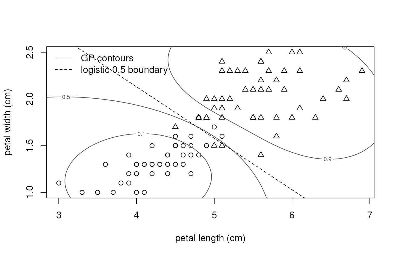
The two classifiers misclassify the same 6 flowers, and where the classes overlap the classifier’s 0.5 contour follows the logistic boundary. The latent function has a large variance because the classes are nearly separable, so its probability changes quickly across the overlap, as the logistic regression’s does. The logistic regression has the lower training log loss: its probabilities are more extreme, which pays on the correctly classified flowers. The Gaussian process’s are closer to 0.5, which pays on the misclassified ones. Neither number measures out-of-sample performance.
Away from the data the two models differ in kind. The logistic
regression extends its linear trend. The Gaussian process returns to its
prior mean, here the estimated intercept 2.71, a probability of 0.94 for
virginica, so its 0.5 contour curves round the versicolor flowers
instead of continuing the boundary. That is the stationary kernel’s
prior, not information in the data; a linear mean
(linear_mean()) would extrapolate like the logistic
regression.
Reproduction: counts of great discoveries
datasets::discoveries counts the “great” inventions and
scientific discoveries in each year from 1860 to 1959. The canonical
analysis is a Poisson regression with a quadratic trend in the year. A
Poisson model with a latent Gaussian process, a Matérn-5/2 kernel, and
an estimated intercept lets the rate vary without a parametric form.
year <- as.numeric(stats::time(datasets::discoveries))
count <- as.numeric(datasets::discoveries)

counts_model <- optimize_latent_gp(
  year,
  count,
  kernel = matern52_kernel(variance = 0.3, length_scale = 20),
  likelihood = poisson_likelihood(),
  mean = constant_mean(estimate_coefficients()),
  n_starts = 3
)
quadratic <- stats::glm(count ~ stats::poly(year, 2),
                        family = stats::poisson())

counts_model$optimization$optimized_parameters
#>       variance   length_scale mean.intercept
#>      0.1659194      3.4199238      1.0367935

rate <- predict_latent_gp(counts_model, year)
pearson_dispersion <- c(
  gp = sum((count - rate$response_mean)^2 / rate$response_mean) /
    length(count),
  quadratic = sum(stats::residuals(quadratic, type = "pearson")^2) /
    stats::df.residual(quadratic)
)
pearson_dispersion
#>        gp quadratic
#> 0.7870345 1.3056491
plot(year, count, pch = 16, cex = 0.6, col = "grey40",
     xlab = "year", ylab = "discoveries")
polygon(c(year, rev(year)),
        c(rate$rate_interval[, "lower"], rev(rate$rate_interval[, "upper"])),
        col = grDevices::adjustcolor("steelblue", 0.25), border = NA)
lines(year, exp(rate$mean), col = "steelblue", lwd = 2)
lines(year, stats::fitted(quadratic), lty = 2, lwd = 2)
legend("topright", legend = c("GP rate (median, 95% interval)",
                              "quadratic Poisson regression"),
       lty = c(1, 2), col = c("steelblue", "black"), lwd = 2, bty = "n")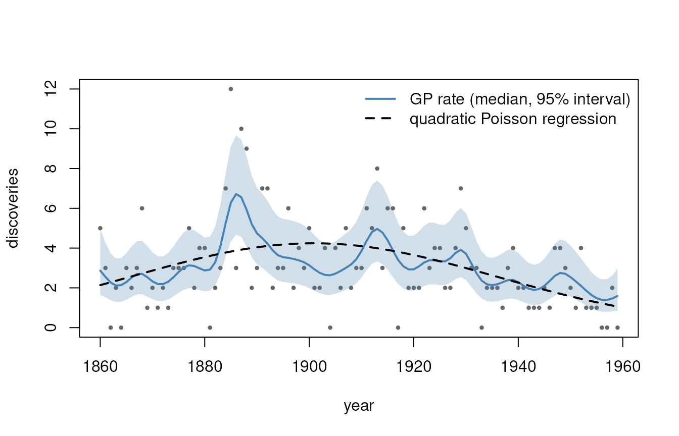
The estimated length scale, 3.4 years, is short: the Gaussian process finds variation in the rate within a decade, such as the peak in the mid-1880s, which the quadratic trend smooths over. The quadratic regression’s Pearson statistic is 1.31 times its residual degrees of freedom, the usual sign of overdispersion around its trend. The Gaussian process attributes that variation to the rate: around its fitted rate the Pearson statistic per year is 0.79, below 1, as it is for any rate fitted to the same counts. Both models describe a rise and a later decline. The quadratic trend leaves the 95% interval of the Gaussian process’s rate only in 1885-1888, 1904, 1948-1949: the other swings are within what the counts leave uncertain.