Draw functions from a Gaussian-process posterior — sample_gp_posterior.gaussianprocesses_latent

Draws latent function values from the posterior of a fitted model and, optionally, noisy observations from the posterior predictive distribution.

Usage

# S3 method for class 'gaussianprocesses_latent_model'
sample_gp_posterior(
  model,
  x,
  n_draws = 1L,
  type = c("latent", "observation"),
  seed = NULL,
  exposure = NULL,
  initial_jitter = 0,
  fallback_jitter = 1e-10,
  jitter_multiplier = 10,
  max_attempts = 8L,
  symmetry_tolerance = sqrt(.Machine$double.eps),
  ...
)

sample_gp_posterior(model, x, n_draws = 1L, ...)

# Default S3 method
sample_gp_posterior(model, x, n_draws = 1L, ...)

# S3 method for class 'gaussianprocesses_model'
sample_gp_posterior(
  model,
  x,
  n_draws = 1L,
  type = c("latent", "observation"),
  observation_noise_variance = NULL,
  seed = NULL,
  initial_jitter = 0,
  fallback_jitter = 1e-10,
  jitter_multiplier = 10,
  max_attempts = 8L,
  symmetry_tolerance = sqrt(.Machine$double.eps),
  ...
)

# S3 method for class 'gaussianprocesses_heteroscedastic_model'
sample_gp_posterior(
  model,
  x,
  n_draws = 1L,
  type = c("latent", "observation"),
  seed = NULL,
  initial_jitter = 0,
  fallback_jitter = 1e-10,
  jitter_multiplier = 10,
  max_attempts = 8L,
  symmetry_tolerance = sqrt(.Machine$double.eps),
  ...
)

# S3 method for class 'gaussianprocesses_sparse_model'
sample_gp_posterior(
  model,
  x,
  n_draws = 1L,
  type = c("latent", "observation"),
  observation_noise_variance = NULL,
  seed = NULL,
  initial_jitter = 0,
  fallback_jitter = 1e-10,
  jitter_multiplier = 10,
  max_attempts = 8L,
  symmetry_tolerance = sqrt(.Machine$double.eps),
  ...
)

# S3 method for class 'gaussianprocesses_state_space_model'
sample_gp_posterior(
  model,
  x,
  n_draws = 1L,
  type = c("latent", "observation"),
  observation_noise_variance = NULL,
  seed = NULL,
  ...
)

Arguments

model: A fitted gaussianprocesses_model (from fit_gp(), optimize_gp(), or fit_time_series_gp()), a gaussianprocesses_heteroscedastic_model (from fit_heteroscedastic_gp()), a gaussianprocesses_latent_model (from fit_latent_gp() or optimize_latent_gp()), or a gaussianprocesses_sparse_model (from fit_sparse_gp() or optimize_sparse_gp()).
x: Numeric vector or matrix of prediction inputs. For models fitted with fit_time_series_gp(), use the numeric time index.
n_draws: Number of independent draws.
type: "latent" draws the latent function \(f(x)\). "observation" also draws noisy observations \(y = f(x) + \varepsilon\); both are returned, with the observations generated from the same latent draws.
seed: Optional non-negative integer seed. The caller's random state is restored afterwards.
exposure: For latent Poisson models, optional exposure of the observation draws, as in predict_latent_gp().
initial_jitter: Non-negative jitter tried first, relative to the covariance scale (the mean of its diagonal).
fallback_jitter: Positive relative jitter tried after the first failed factorization.
jitter_multiplier: Multiplicative jitter escalation factor.
max_attempts: Maximum Cholesky attempts.
symmetry_tolerance: Relative tolerance for checking that the covariance matrix is symmetric.
...: Further arguments passed to methods.
observation_noise_variance: For exact and sparse models, optional non-negative scalar or vector of noise variances at x, used only when type = "observation". It defaults to the fitted noise variance of homoscedastic models and is required for models fitted with observation-specific noise.

Value

An object of class gaussianprocesses_samples with one row per input point and one column per draw in latent and, for type = "observation", in observation. It also contains the posterior mean, the latent_covariance that was sampled, the observation_noise_variance used for observation draws, the numerical jitter with its relative_jitter and covariance_scale, and the cholesky_attempts.

Details

The posterior mean \(\mu\) and latent covariance \(\Sigma\) come from predict_gp() (or predict_heteroscedastic_gp()), which uses triangular solves with the fitted Cholesky factor; no covariance matrix is inverted. Latent draws are \(\mu + R^\top z\) with \(\Sigma = R^\top R\) and \(z \sim \mathcal{N}(0, I)\). Posterior covariances are often nearly singular, for example at closely spaced or repeated inputs; the factor then uses the package's jitter policy, and the jitter is reported.

Observation draws add independent noise, \(y = f + \varepsilon\) with \(\varepsilon \sim \mathcal{N}(0, \mathrm{diag}(\sigma^2_*))\), so their covariance is \(\Sigma + \mathrm{diag}(\sigma^2_*)\).

For heteroscedastic models, the latent draws come from the mean GP and the noise variances \(\sigma^2_*\) are the plug-in estimates of predict_heteroscedastic_gp(). The draws are therefore conditional on the estimated noise function: uncertainty in the noise process is not propagated, consistent with the approximation being a plug-in method rather than full Bayesian inference.

For latent models, the latent draws come from the Gaussian (Laplace) approximation of predict_latent_gp(), and observation draws are drawn from the likelihood given each latent draw: Bernoulli, Poisson (with exposure), or Gaussian responses. Their observation_noise_variance is NULL. For Bernoulli likelihoods the samples also contain probability, the class probability \(\pi(f)\) of each latent draw, whose mean over draws is the predictive probability of predict_latent_gp(); for Poisson likelihoods they contain rate, the rate \(E e^f\) of each latent draw.

For sparse models (FITC or VFE, fit_sparse_gp()), the draws use the sparse posterior covariance \(K_{**} - Q_{**} + K_{*u} A^{-1} K_{u*}\) of predict_sparse_gp() at the \(k\) sampling inputs. It costs \(O(k m^2 + k^2 m)\) time for \(m\) inducing points, and its factorization \(O(k^3)\) time and \(O(k^2)\) memory, as for exact models. The number of inducing points enters only through \(m \times k\) cross-covariances, so the limit is the number of sampling inputs, a few thousand, rather than \(m\). Observation draws need observation_noise_variance for models fitted with observation-specific noise.

Stability

Stable: from version 1.0.0 this interface changes incompatibly only in a major release, after a deprecation period. Results and options that concern an experimental model class, kernel, or argument follow that interface's tier. See gaussianprocesses-package for the policy.

Examples

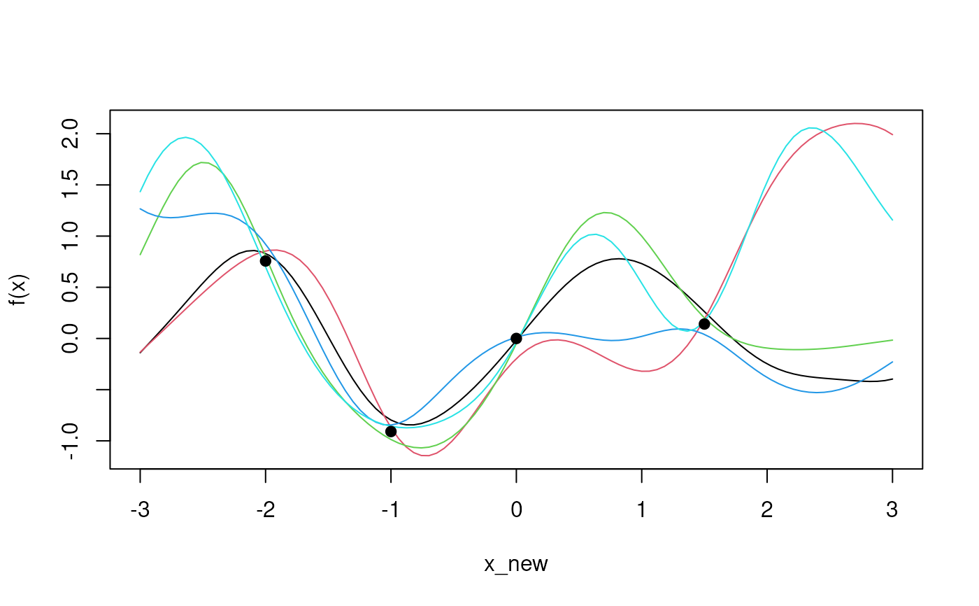
x <- c(-2, -1, 0, 1.5)
y <- sin(2 * x)
model <- fit_gp(x, y, rbf_kernel(length_scale = 0.7), noise_variance = 0.01)

x_new <- seq(-3, 3, length.out = 100)
draws <- sample_gp_posterior(model, x_new, n_draws = 5, seed = 1)
draws
#> Gaussian-process samples
#>   distribution: posterior (exact)
#>   draws: 5 at 100 input point(s)
#>   contents: latent function draws
#>   numerical jitter: 2.89e-11 (1e-10 times the covariance scale 0.289)

matplot(x_new, draws$latent, type = "l", lty = 1, ylab = "f(x)")
points(x, y, pch = 19)


# Noisy observation draws are generated from the same latent draws.
noisy <- sample_gp_posterior(
  model,
  x_new,
  n_draws = 1,
  type = "observation",
  seed = 2
)
head(cbind(latent = noisy$latent[, 1], observation = noisy$observation[, 1]))
#>           latent observation
#> [1,] -0.38953043 -0.28208448
#> [2,] -0.30355747 -0.27749768
#> [3,] -0.19821462 -0.22964181
#> [4,] -0.07810449 -0.15306750
#> [5,]  0.05161452 -0.03460532
#> [6,]  0.18550856  0.39031259