Marginal Likelihood, Prediction, and Uncertainty • gaussianprocesses

Marginal likelihood

For centered observations

\tilde y = y-m(X)

and observation covariance

C=K(X,X)+\Sigma_\varepsilon,

the log marginal likelihood is

\log p(y\mid X,\theta) = -\frac{1}{2}\tilde y^\top C^{-1}\tilde y -\frac{1}{2}\log |C| -\frac{n}{2}\log(2\pi).

C=R^\top R,

then

\log|C| = 2\sum_{i=1}^n\log R_{ii}.

The implementation uses exactly this form:

x <- seq(-1.5, 1.5, length.out = 12)
y <- sin(2 * x) + 0.1 * x

initial_kernel <- rbf_kernel(
  variance = 0.5,
  length_scale = 1.5
)

initial_model <- fit_gp(
  x,
  y,
  kernel = initial_kernel,
  noise_variance = 0.05
)

log_marginal_likelihood(initial_model)
#> [1] -12.87926

Hyperparameter estimation

Positive kernel parameters are optimized in log space.

If \theta_j>0, define

\eta_j = \log\theta_j.

Optimization then proceeds over unconstrained or bounded \eta_j, while the kernel continues to store parameters on their natural scale. L-BFGS-B uses the exact gradient from log_marginal_likelihood_gradient(), derived in the vignette on hyperparameter derivatives.

optimized <- optimize_gp(
  x,
  y,
  kernel = initial_kernel,
  noise_variance = 0.05,
  optimize_noise = TRUE,
  n_starts = 2,
  control = list(maxit = 30)
)

kernel_parameters(
  optimized$kernel,
  flatten = TRUE
)
#>     variance length_scale 
#>     3.537301     1.296346

optimized$noise_variance
#> [1] 1e-08
optimized$optimization$log_marginal_likelihood
#> [1] 32.8508

The optimizer retains diagnostics rather than returning only a parameter vector:

optimized$optimization[c(
  "method",
  "converged",
  "best_start",
  "counts"
)]
#> $method
#> [1] "L-BFGS-B"
#> 
#> $converged
#> [1] TRUE
#> 
#> $best_start
#> [1] 2
#> 
#> $counts
#> function gradient 
#>       39       39

Posterior uncertainty

For a test point x_*,

\operatorname{Var}[f_*\mid y] = k(x_*,x_*) - k_{*f}C^{-1}k_{f*}.

This is latent-function uncertainty.

For a future noisy observation,

\operatorname{Var}[y_*\mid y] = \operatorname{Var}[f_*\mid y] + \sigma_*^2.

The package reports both:

x_new <- seq(-2, 2, length.out = 25)

prediction <- predict_gp(
  optimized,
  x_new,
  interval_level = 0.9
)

head(
  data.frame(
    x = x_new,
    mean = prediction$mean,
    latent_variance = prediction$latent_variance,
    observation_variance = prediction$observation_variance
  )
)
#>           x        mean latent_variance observation_variance
#> 1 -2.000000  0.57084819    1.673447e-04         1.673547e-04
#> 2 -1.833333  0.32278691    2.177748e-05         2.178748e-05
#> 3 -1.666667  0.02497712    1.294242e-06         1.304242e-06
#> 4 -1.500000 -0.29111734    9.989469e-09         1.998947e-08
#> 5 -1.333333 -0.59068237    1.888936e-08         2.888936e-08
#> 6 -1.166667 -0.83973602    7.398821e-09         1.739882e-08

Exact leave-one-out diagnostics

Let

Q=C^{-1}

and

\alpha=Q\tilde y.

The exact leave-one-out predictive distribution can be recovered without refitting n models:

\mu_{-i} = y_i - \frac{\alpha_i}{Q_{ii}},

\sigma_{-i}^2 = \frac{1}{Q_{ii}}.

That is the basis of loo_gp():

loo <- loo_gp(optimized)

head(loo)
#>   observation   observed       mean     variance           sd      residual
#> 1           1 -0.2911200 -0.2885900 9.496945e-06 0.0030817113 -2.530057e-03
#> 2           2 -0.7569843 -0.7573858 3.104270e-07 0.0005571598  4.014965e-04
#> 3           3 -1.0387766 -1.0386418 5.170449e-08 0.0002273862 -1.348082e-04
#> 4           4 -1.0468008 -1.0468659 2.568663e-08 0.0001602705  6.503314e-05
#> 5           5 -0.7708133 -0.7708020 2.523363e-08 0.0001588510 -1.133145e-05
#> 6           6 -0.2829953 -0.2829533 2.366410e-08 0.0001538314 -4.197755e-05
#>   standardized_residual       pit      lower      upper covered
#> 1           -0.82099077 0.2058258 -0.2946300 -0.2825499    TRUE
#> 2            0.72061278 0.7644261 -0.7584779 -0.7562938    TRUE
#> 3           -0.59286023 0.2766373 -1.0390874 -1.0381961    TRUE
#> 4            0.40577109 0.6575446 -1.0471800 -1.0465517    TRUE
#> 5           -0.07133385 0.4715660 -0.7711133 -0.7704906    TRUE
#> 6           -0.27288022 0.3924726 -0.2832548 -0.2826518    TRUE
#>   log_predictive_density
#> 1               4.526319
#> 2               6.314079
#> 3               7.294180
#> 4               7.737384
#> 5               7.826061
#> 6               7.823483

Calibration summaries are descriptive rather than binary tests:

gp_calibration_diagnostics(
  optimized,
  interval_level = 0.9
)
#> $interval_level
#> [1] 0.9
#> 
#> $empirical_coverage
#> [1] 1
#> 
#> $coverage_error
#> [1] 0.1
#> 
#> $mean_standardized_residual
#> [1] -8.211022e-10
#> 
#> $sd_standardized_residual
#> [1] 0.5703259
#> 
#> $mean_absolute_standardized_residual
#> [1] 0.4807415
#> 
#> $pit_mean
#> [1] 0.5
#> 
#> $pit_variance
#> [1] 0.04428026
#> 
#> $mean_log_predictive_density
#> [1] 6.920251

The same separation applies throughout the package: predictive calibration, model structure, and numerical conditioning are related, but they are not the same object.

Universal kriging

A zero or fixed mean says that, far from the data, the function returns to a known level. Often the data follow a trend instead. Universal kriging writes the mean as a regression on known basis functions,

f(x) = h(x)^\top \beta + g(x), \qquad g \sim \mathcal{GP}(0, k),

with H the matrix whose rows are h(x_i)^\top. linear_mean(), polynomial_mean(), and basis_mean() define h. The coefficients \beta can be treated in three ways, and the choice changes both the hyperparameter estimates and the predictive uncertainty.

Estimated. For given hyperparameters, the generalized least-squares estimate

\hat\beta = (H^\top C^{-1} H)^{-1} H^\top C^{-1} y

maximizes the likelihood. Substituting it gives the profile likelihood (estimate_coefficients("ml"), the default). The profile likelihood ignores that p degrees of freedom went into \hat\beta, so, as with the maximum-likelihood variance of a linear regression, it underestimates variances. The restricted likelihood (estimate_coefficients("reml")) is the likelihood of the residuals after projecting out the trend:

\ell_R = -\tfrac12 y^\top P y - \tfrac12 \log|C| - \tfrac12 \log|H^\top C^{-1} H| - \tfrac{n - p}{2} \log 2\pi, \qquad P = C^{-1} - C^{-1} H (H^\top C^{-1} H)^{-1} H^\top C^{-1}.

Predictions plug in \hat\beta as if it were known.

Marginalized. A Gaussian prior \beta \sim N(b, B) (coefficient_prior(b, B)) makes the model a Gaussian process with mean h(x)^\top b and covariance k(x, x') + h(x)^\top B h(x'). Its predictive covariance adds the uncertainty of \beta,

R_* (B^{-1} + H^\top C^{-1} H)^{-1} R_*^\top, \qquad R_* = H_* - K_{*X} C^{-1} H,

which grows where the prediction relies on the trend: away from the data. coefficient_prior() without a covariance takes the vague limit B^{-1} \to 0. Its predictive mean is the plug-in mean with \hat\beta, and its likelihood is the restricted likelihood.

Fixed. A numeric vector, linear_mean(c(2, 0.8)), fixes \beta.

The implementation never forms (H^\top C^{-1} H)^{-1}. It solves the generalized least-squares problem with the QR decomposition of the whitened basis R^{-\top} H, where C = R^\top R, and a basis whose coefficients are not identified raises an error of class gaussianprocesses_rank_deficiency_error.

Simulate a linear trend with a smooth deviation, observed on [0, 10]:

set.seed(26)
x_trend <- sort(runif(30, 0, 10))
truth <- function(x) 2 + 0.8 * x + sin(1.3 * x)
y_trend <- truth(x_trend) + rnorm(30, sd = 0.2)

fit_with_mean <- function(mean) {
  optimize_gp(
    x_trend,
    y_trend,
    kernel = rbf_kernel(variance = 1, length_scale = 1),
    noise_variance = 0.05,
    mean = mean
  )
}

trend_models <- list(
  "zero mean" = fit_with_mean(zero_mean()),
  "estimated, ML" = fit_with_mean(linear_mean()),
  "estimated, REML" = fit_with_mean(
    linear_mean(estimate_coefficients("reml"))
  ),
  "vague prior" = fit_with_mean(linear_mean(coefficient_prior()))
)

data.frame(
  likelihood = sapply(trend_models, function(model) {
    model$optimization$likelihood
  }),
  variance = sapply(trend_models, function(model) {
    model$kernel$parameters$variance
  }),
  length_scale = sapply(trend_models, function(model) {
    model$kernel$parameters$length_scale
  })
)
#>                 likelihood   variance length_scale
#> zero mean         marginal 35.8387340    2.3087250
#> estimated, ML      profile  0.3926470    0.8395031
#> estimated, REML restricted  0.5695221    0.9090621
#> vague prior     restricted  0.5695221    0.9090621

Without a trend, the kernel has to explain it: the variance and length scale are large. REML estimates a larger kernel variance than the profile likelihood. The vague prior maximizes the same restricted likelihood, so it reaches the same estimates.

coef() and vcov() give the coefficients and their covariance for given hyperparameters:

estimated <- trend_models[["estimated, REML"]]

cbind(
  estimate = coef(estimated),
  standard_error = sqrt(diag(vcov(estimated)))
)
#>           estimate standard_error
#> intercept 1.976234     0.59687649
#> x1        0.816017     0.09783671

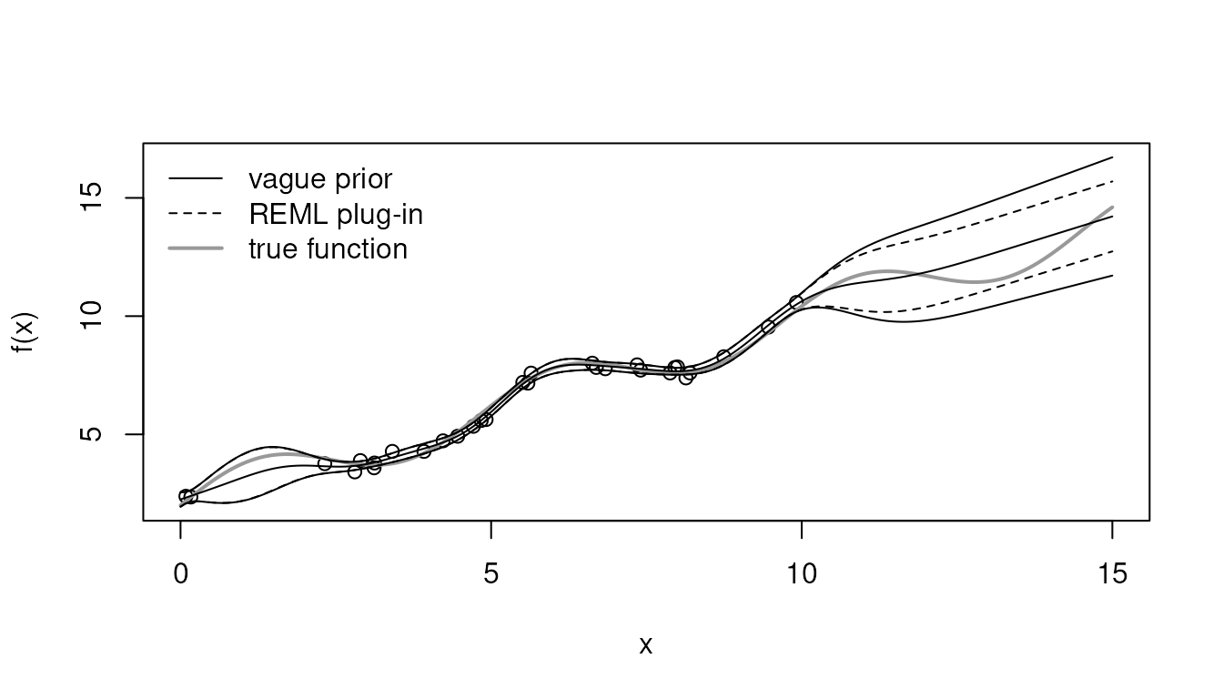
The models differ most when they extrapolate. At x = 15 the true value is 14.61:

t(sapply(trend_models, function(model) {
  prediction <- predict_gp(model, 15)
  c(mean = prediction$mean, latent_sd = prediction$latent_sd)
}))
#>                     mean latent_sd
#> zero mean        1.88379 5.8170262
#> estimated, ML   14.16448 0.6266155
#> estimated, REML 14.21649 0.7546669
#> vague prior     14.21649 1.2762504

The zero-mean model returns towards zero with a large standard deviation. The trend models follow the trend. The REML and vague-prior models have the same hyperparameters and the same mean, but only the vague prior includes the uncertainty of the slope, which grows with the distance from the data:

x_grid <- seq(0, 15, length.out = 200)
plug_in <- predict_gp(trend_models[["estimated, REML"]], x_grid)
marginal <- predict_gp(trend_models[["vague prior"]], x_grid)

plot(
  x_trend,
  y_trend,
  xlim = c(0, 15),
  ylim = range(marginal$latent_interval, y_trend),
  xlab = "x",
  ylab = "f(x)"
)
lines(x_grid, truth(x_grid), col = "grey60", lwd = 2)
lines(x_grid, marginal$mean)
matlines(x_grid, marginal$latent_interval, lty = 1, col = "black")
matlines(x_grid, plug_in$latent_interval, lty = 2, col = "black")
legend(
  "topleft",
  legend = c("vague prior", "REML plug-in", "true function"),
  lty = c(1, 2, 1),
  col = c("black", "black", "grey60"),
  lwd = c(1, 1, 2),
  bty = "n"
)

Latent 95% intervals over x from 0 to 15 for the REML plug-in model (dashed lines) and the vague-prior model (solid lines), with the data as points on 0 to 10 and the true function as a grey line. The two intervals coincide over the data and the vague-prior interval becomes wider beyond x = 10.

Leave-one-out predictions follow the same treatment: with marginalized coefficients, loo_gp() re-estimates the trend without each observation; with estimated coefficients, it keeps the full-data estimate.