Gaussian Processes for Time Series

Time is an input, not a special likelihood

For a one-dimensional time series, a Gaussian process can be written as

f(t)\sim\mathcal{GP}(m(t),k(t,t')).

The important modelling choice is therefore the covariance structure.

Time ordering is not silently inferred by the package. It is validated explicitly.

time <- as.Date("2026-01-01") + 0:9

index <- gp_time_index(time)

index
#>  [1] 0 1 2 3 4 5 6 7 8 9
#> attr(,"origin")
#> [1] "2026-01-01"
#> attr(,"unit")
#> [1] "days"
#> attr(,"input_type")
#> [1] "Date"
#> attr(,"class")
#> [1] "gaussianprocesses_time_index" "numeric"
attributes(index)[c("origin", "unit", "input_type")]
#> $origin
#> [1] "2026-01-01"
#> 
#> $unit
#> [1] "days"
#> 
#> $input_type
#> [1] "Date"

Non-increasing time values are rejected rather than silently sorted.

Trend, periodicity, and local variation

A useful additive model is

k(t,t') = k_{\text{trend}}(t,t') + k_{\text{periodic}}(t,t') + k_{\text{local}}(t,t').

The convenience constructor makes this structure explicit:

kernel <- time_series_kernel(
  period = 12,
  trend_variance = 0.03,
  periodic_variance = 1,
  periodic_length_scale = 0.8,
  local_variance = 0.25,
  local_length_scale = 2
)

kernel
#> SumKernel(
#>   Linear(variance=0.03)
#>   Periodic(variance=1, length_scale=0.8, period=12)
#>   Matern-3/2(variance=0.25, length_scale=2)
#> )

The linear component is nonstationary. Therefore the convenience model does not hide a claim that the full process is stationary.

Reproducible example

time_numeric <- 0:24

response <-
  0.04 * time_numeric +
  sin(2 * pi * time_numeric / 12) +
  0.15 * cos(2 * pi * time_numeric / 3)

model <- fit_time_series_gp(
  time_numeric,
  response,
  kernel = kernel,
  noise_variance = 0.05
)

Interpolation versus extrapolation

Requested times are labelled by their relation to the observed time range:

requested_time <- c(6.5, 18.5, 25, 26, 27)

forecast <- forecast_gp(
  model,
  requested_time,
  interval_level = 0.95
)

data.frame(
  time = requested_time,
  region = forecast$region,
  mean = forecast$mean,
  lower = forecast$prediction_interval[, "lower"],
  upper = forecast$prediction_interval[, "upper"]
)
#>   time        region       mean       lower     upper
#> 1  6.5 interpolation 0.05428375 -0.52357428 0.6321418
#> 2 18.5 interpolation 0.53296146 -0.04502145 1.1109444
#> 3 25.0      forecast 1.44511324  0.46511947 2.4251070
#> 4 26.0      forecast 1.78246861  0.49787230 3.0670649
#> 5 27.0      forecast 2.03583851  0.61116417 3.4605129

Points inside the training interval are interpolation.

Points after the final observation are forward extrapolation, labelled forecast.

The posterior equations are the same in both cases. Their interpretation is not: extrapolation depends much more strongly on the chosen kernel structure.

Rolling-origin evaluation

A time-series model should not be evaluated by randomly shuffling observations.

The package supplies expanding-window rolling-origin evaluation.

For an origin T_j, the training set is

\{(t_i,y_i): i\le T_j\},

and only future observations are scored.

backtest <- rolling_origin_gp(
  time_numeric,
  response,
  kernel = kernel,
  initial_window = 12,
  horizon = 3,
  step = 3,
  noise_variance = 0.05,
  interval_level = 0.9
)

head(backtest)
#> Gaussian-process rolling-origin backtest
#>   forecasts: 6
#>   origins: 2
#>   maximum horizon: 3

The supplied kernel and noise parameters are kept fixed across origins. This prevents future observations from leaking into earlier origins through whole-series retuning.

Point and probabilistic metrics

forecast_metrics(backtest)
#> $n_forecasts
#> [1] 12
#> 
#> $rmse
#> [1] 0.3017888
#> 
#> $mae
#> [1] 0.2292877
#> 
#> $standardized_rmse
#> [1] 0.3832272
#> 
#> $empirical_coverage
#> [1] 1
#> 
#> $interval_level
#> [1] 0.9
#> 
#> $mean_interval_width
#> [1] 2.406712
#> 
#> $mean_log_predictive_density
#> [1] -0.6607537

The returned summaries include point errors and uncertainty-aware quantities:

• RMSE;
• MAE;
• standardized RMSE;
• empirical interval coverage;
• mean interval width;
• mean log predictive density.

These answer different questions. A narrow interval is not useful if coverage is poor, and a good RMSE does not imply calibrated predictive uncertainty.

Structural breaks

A stationary kernel assumes that the series behaves the same way throughout. After a structural break, a new level, a new seasonal pattern, or a new volatility, that assumption is wrong, and it is wrong in the direction that matters most for forecasting: the data after the break are the only information about the future.

changepoint_kernel() switches between two kernels around a location c with the sigmoid s(t) = 1 / (1 + e^{-a (t - c)}):

k(t, t') = (1 - s(t))\, k_1(t, t')\, (1 - s(t')) + s(t)\, k_2(t, t')\, s(t').

The two regimes are independent processes: as the steepness a grows, times on opposite sides of c become uncorrelated. Each term has the form g(t) k(t, t') g(t'), so the kernel is positive semidefinite. The location and the steepness are hyperparameters, estimated with the others.

Simulate 90 daily observations with a break on 15 March: before it, a slow oscillation around zero; after it, a new level of 2.5 with a weekly pattern.

set.seed(28)
dates <- as.Date("2026-01-01") + 0:89
day <- as.numeric(gp_time_index(dates))
break_day <- as.numeric(as.Date("2026-03-15") - dates[1])

regime_signal <- function(day) {
  ifelse(
    day < break_day,
    sin(2 * pi * day / 30),
    2.5 + 0.4 * sin(2 * pi * day / 7)
  )
}
observed <- regime_signal(day) + rnorm(90, sd = 0.15)

Each regime gets a slowly varying level and a local component. The changepoint model has one copy of this kernel per regime:

regime <- function() {
  sum_kernel(
    rbf_kernel(variance = 1, length_scale = 60),
    matern52_kernel(variance = 0.5, length_scale = 5)
  )
}

single <- optimize_gp(
  day,
  observed,
  kernel = regime(),
  noise_variance = 0.05
)
changing <- optimize_gp(
  day,
  observed,
  kernel = changepoint_kernel(regime(), regime(), location = 45),
  noise_variance = 0.05,
  n_starts = 4
)

c(
  single = log_marginal_likelihood(single),
  changepoint = log_marginal_likelihood(changing)
)
#>      single changepoint 
#>  -30.060432    1.576984

The likelihood is often multimodal in the location, so optimize_gp() starts it at evenly spaced quantiles of the time index and bounds it by the training range. The estimate is on the time-index scale, days since the first date, and converts back to a date:

dates[1] + changing$kernel$parameters$location
#> [1] "2026-03-14"

To forecast, refit both models with fit_time_series_gp() and the estimated parameters, which records the dates:

single_model <- fit_time_series_gp(
  dates,
  observed,
  kernel = single$kernel,
  noise_variance = single$noise_variance
)
changepoint_model <- fit_time_series_gp(
  dates,
  observed,
  kernel = changing$kernel,
  noise_variance = changing$noise_variance
)

future <- max(dates) + c(1, 7, 14, 21)
single_forecast <- forecast_gp(single_model, future)
changepoint_forecast <- forecast_gp(changepoint_model, future)

data.frame(
  date = future,
  truth = regime_signal(as.numeric(future - dates[1])),
  single = single_forecast$mean,
  single_sd = single_forecast$latent_sd,
  changepoint = changepoint_forecast$mean,
  changepoint_sd = changepoint_forecast$latent_sd
)
#>         date    truth    single single_sd changepoint changepoint_sd
#> 1 2026-04-01 2.187267 2.1146728 0.3314075    2.361446      0.2539727
#> 2 2026-04-07 2.110029 1.2834598 0.8130878    2.538680      0.3814787
#> 3 2026-04-14 2.110029 0.4686915 1.2406255    2.539052      0.3815886
#> 4 2026-04-21 2.110029 0.0931824 1.3450361    2.539052      0.3815888

grid <- seq(min(dates), max(dates) + 21, by = 1)
single_path <- forecast_gp(single_model, grid)
changepoint_path <- forecast_gp(changepoint_model, grid)

plot(
  dates,
  observed,
  xlim = range(grid),
  ylim = range(
    single_path$latent_interval,
    changepoint_path$latent_interval,
    observed
  ),
  xlab = "date",
  ylab = "series"
)
abline(v = as.Date("2026-03-15"), col = "grey60", lty = 3)
lines(grid, changepoint_path$mean)
matlines(grid, changepoint_path$latent_interval, lty = 1, col = "grey40")
lines(grid, single_path$mean, lty = 2)
matlines(grid, single_path$latent_interval, lty = 2, col = "grey40")
legend(
  "topleft",
  legend = c("changepoint", "single kernel"),
  lty = c(1, 2),
  bty = "n"
)

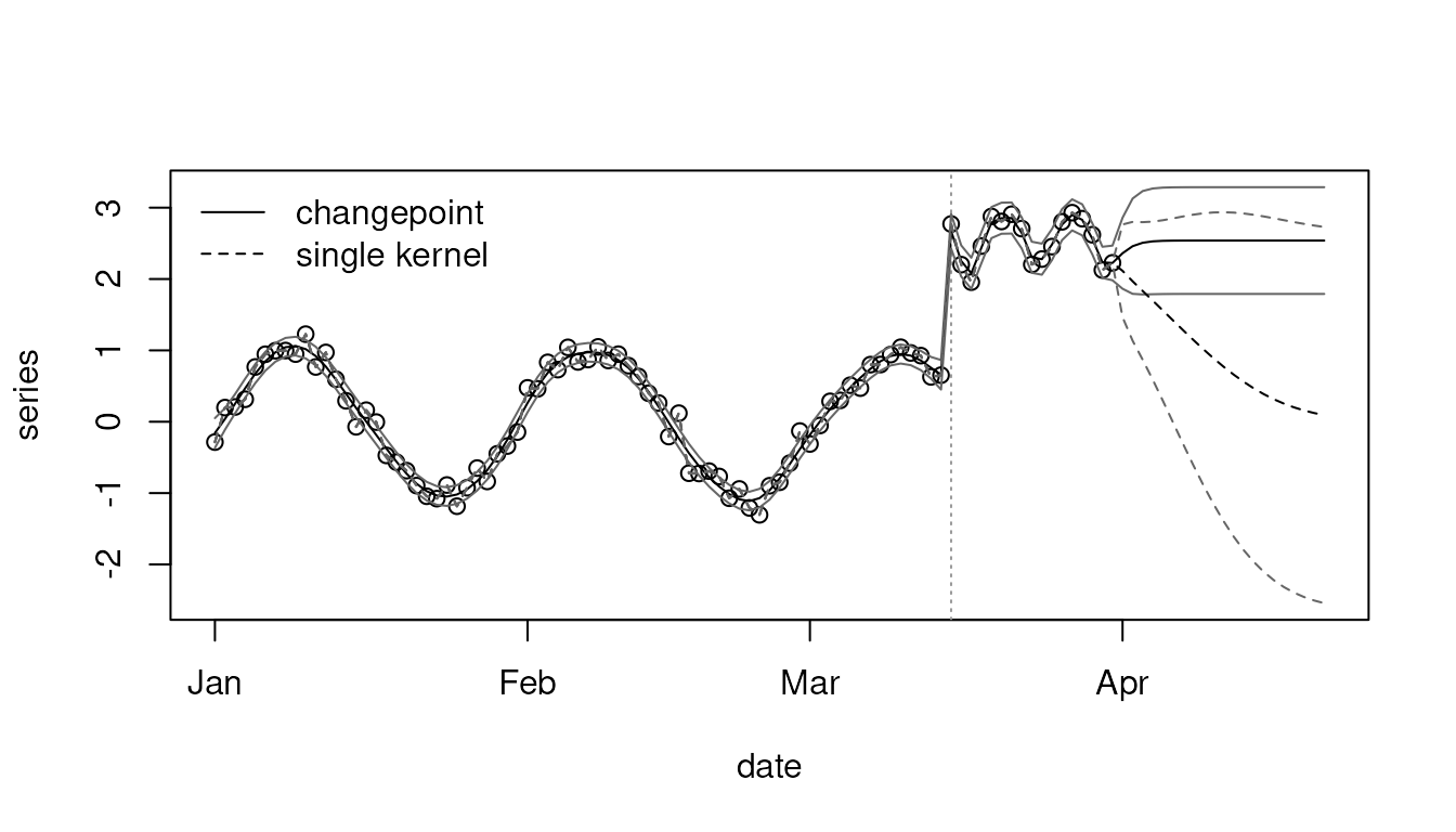
The single kernel has to explain a jump of 2.5 with one covariance. It does so with short-memory variation, and its forecast falls back towards zero over the following three weeks while its interval widens. The changepoint model estimates the post-break regime from the 17 days after the break: a persistent new level, with short-memory variation around it. Its forecast stays at that level; the weekly pattern is too short-lived in its estimated kernel to carry forward. Its uncertainty reflects only how much those 17 days determine.

Some caveats:

• The location is a point estimate: its uncertainty is not propagated into the forecasts.
• Several breaks come from nesting changepoint kernels, at the cost of more hyperparameters and more local optima.
• time_series_kernel(period, changepoint = c) builds the same structure around the trend-periodic-local kernel, with independent copies before and after the break. To place a break at a date, convert it with gp_time_index(c(dates[1], date))[2].

Long series: Kalman filtering and smoothing

Exact inference factorizes the n \times n covariance matrix of the observations, which costs O(n^3) time and O(n^2) memory: a few thousand observations are the practical limit. For time series there is an exact shortcut. On one input, a Matérn process with \nu = p + \tfrac12 is the first component of the state x(t) = (f(t), f'(t), \ldots, f^{(p)}(t)) of a linear stochastic differential equation

\mathrm{d}x = F x\,\mathrm{d}t + L\,\mathrm{d}W,

where F is a (p + 1) \times (p + 1) matrix fixed by the length scale and W is white noise whose intensity is fixed by the variance (Hartikainen and Särkkä, 2010). Observed at sorted times, the process is a linear Gaussian state-space model: the state moves from one time to the next by the matrix exponential e^{F \Delta t}, and each observation is the first state component plus noise. The Kalman filter then computes the log marginal likelihood from one-step prediction errors, and the Rauch-Tung-Striebel smoother computes the posterior, in O(n) time. This is not an approximation: it is the same Gaussian posterior, computed in a different order.

fit_time_series_gp(method = "state_space") uses it for Matérn-1/2, 3/2, and 5/2 kernels, their sums, and scaled versions of them. Fit 1500 irregularly spaced observations both ways:

set.seed(3)
long_time <- sort(runif(1500, 0, 300))
long_y <- sin(2 * pi * long_time / 50) + 0.3 * sin(long_time / 3) +
  rnorm(1500, sd = 0.2)
long_kernel <- sum_kernel(
  matern52_kernel(variance = 1, length_scale = 15),
  matern12_kernel(variance = 0.1, length_scale = 2)
)

exact_long <- fit_time_series_gp(
  long_time,
  long_y,
  kernel = long_kernel,
  noise_variance = 0.04
)
kalman_long <- fit_time_series_gp(
  long_time,
  long_y,
  kernel = long_kernel,
  noise_variance = 0.04,
  method = "state_space"
)

c(exact = logLik(exact_long), state_space = logLik(kalman_long))
#>       exact state_space 
#>    29.78026    29.78026

Forecasts are computed by placing the requested times among the training times as steps without an observation, so they cost O(n + m) for m requested times:

requested_long <- c(-5, 150.25, 299.9, 305, 330)
exact_forecast <- forecast_gp(exact_long, requested_long)
kalman_forecast <- forecast_gp(kalman_long, requested_long)

data.frame(
  time = requested_long,
  region = kalman_forecast$region,
  exact_mean = exact_forecast$mean,
  state_space_mean = kalman_forecast$mean,
  exact_sd = exact_forecast$observation_sd,
  state_space_sd = kalman_forecast$observation_sd
)
#>     time                 region   exact_mean state_space_mean  exact_sd
#> 1  -5.00 backward_extrapolation -0.131140250     -0.131140250 0.6140062
#> 2 150.25          interpolation -0.018190832     -0.018190832 0.2661293
#> 3 299.90          interpolation -0.068115710     -0.068115710 0.2319000
#> 4 305.00               forecast  0.008434929      0.008434929 0.5996931
#> 5 330.00               forecast  0.070838157      0.070838157 1.0579626
#>   state_space_sd
#> 1      0.6140062
#> 2      0.2661293
#> 3      0.2319000
#> 4      0.5996931
#> 5      1.0579626

c(
  mean = max(abs(kalman_forecast$mean - exact_forecast$mean)),
  sd = max(abs(kalman_forecast$observation_sd - exact_forecast$observation_sd))
)
#>         mean           sd 
#> 1.376677e-14 5.551115e-16

The two methods agree to rounding error. The package’s tests check the log marginal likelihood, posterior means, and posterior variances against the exact GP to a relative 10^{-8} for each supported kernel, on irregular and tied inputs. predict(), logLik(), fitted(), and rolling_origin_gp(method = "state_space") work as for exact models, and sample_gp_posterior() draws by forward filtering, backward sampling.

Kernels without a finite-dimensional state, such as the RBF, periodic, linear, and rational quadratic kernels and products of kernels, are refused. In particular time_series_kernel(), which has linear and periodic components, needs method = "exact":

tryCatch(
  fit_time_series_gp(
    time_numeric,
    response,
    kernel = kernel,
    noise_variance = 0.05,
    method = "state_space"
  ),
  gaussianprocesses_state_space_error = conditionMessage
)
#> [1] "The Linear kernel has no exact state-space representation; use method = \"exact\". Matern-1/2, 3/2, and 5/2 kernels, their sums, and scaled versions have one."

optimize_time_series_gp() estimates the hyperparameters with either method. With method = "state_space" each objective value is one filter pass, and the optimizer approximates gradients by finite differences:

first <- seq_len(300)
kalman_fit <- optimize_time_series_gp(
  long_time[first],
  long_y[first],
  kernel = matern52_kernel(length_scale = 10),
  noise_variance = 0.1,
  n_starts = 1,
  method = "state_space"
)
exact_fit <- optimize_time_series_gp(
  long_time[first],
  long_y[first],
  kernel = matern52_kernel(length_scale = 10),
  noise_variance = 0.1,
  n_starts = 1
)

rbind(
  exact = exact_fit$optimization$optimized_parameters,
  state_space = kalman_fit$optimization$optimized_parameters
)
#>             variance length_scale noise_variance
#> exact       1.177376     12.85724     0.04011387
#> state_space 1.177368     12.85721     0.04011387

The cost grows linearly in the number of observations. inst/benchmarks/state-space-scaling.R times both methods on irregular series, as the median of three runs in fresh R processes on a desktop machine. With a Matérn-5/2 kernel, fitting 5000 observations took 0.18 seconds by Kalman smoothing and 28 seconds by exact inference; 100 000 observations took 3.6 seconds, where exact inference would need 80 GB for the covariance matrix alone. Between 1000 and 100 000 observations the log-log slope of the fitting time was 1.02 (0.96 for the sum of a Matérn-5/2 and a Matérn-1/2 kernel), against 3.1 to 3.4 for exact inference between 1000 and 5000. One filter pass, the cost of one objective value during optimization, took about 17 microseconds per observation.